The Buy-to-Build Indicator
New Estimates and Comment
Joseph Francis, Shimshon Bichler and Jonathan Nitzan [*]
London, Jerusalem and Montreal, March-April 2013
![]()
The first part of the exchange is a short article by Joseph Francis. The article provides new estimates and an assessment of the buy-to-build indicator for the United States and Britain. The second part offers commentary by Shimshon Bichler and Jonathan Nitzan.
The Buy-to-Build Indicator: New Estimates for Britain and the United States
Joseph Francis [**]
London School of Economics, March 2013
This note presents new long-term estimates of what Jonathan Nitzan and Shimshon Bichler (2002: 53-4, 82-3; 2009: Ch.15) have named the ‘buy-to-build indicator’, which is calculated as the value of mergers and acquisitions as a percentage of gross capital formation. Estimating the buy-to-build indicators is not simple, principally due to the absence of consistent series for expenditure on mergers and acquisitions. Nevertheless, as this note describes, it has proven possible to calculate them for both Britain and the United States. For Britain, the new estimates build principally on the research of the Leslie Hannah, as well as official government statistics, while for the United States, they represent significant revisions of Nitzan and Bichler’s own original estimates. The note concludes with some observations on the new series.
New Estimates
Britain
Estimating a buy-to-build indicator for Britain is relatively straightforward. Hannah’s (1983: 167-78) series of the value of firm disappearances due to mergers in manufacturing industry during 1880-1939 and 1949-1981 can be easily spliced with the official Office for National Statistics (ONS n.d.: Series DUCM and CBCQ) series of expenditure on mergers, which cover expenditure on mergers in Britain by British companies during 1965-85 and by British and foreign companies in Britain during 1986-2012. The raw data can be seen in part (a) of Figure 1, in which the series for the value of mergers and acquisitions are shown as percentages of gross fixed capital formation,[1] in order to arrive at buy-to-build indicators.
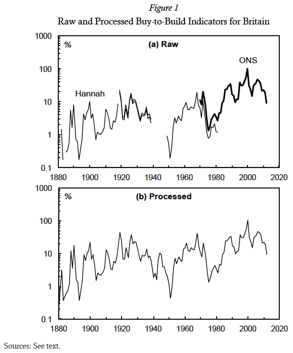
Simple ratio splicing was used to join the Hannah and ONS series. Hannah’s were adjusted upwards according to the average ratio between the two series during 1965-81, in order to roughly compensate for the absence of non-manufacturing mergers and acquisitions in Hannah’s series.[2] The gap in Hannah’s series between 1939 and 1949 was filled through exponential interpolation, adjusted following the variations in a proxy that was construct by multiplying the number of mergers by the Actuaries General Share Price Index, then dividing it by gross fixed capital formation.[3] The continuous buy-to-build indicator that resulted from this processing can be seen in part (b) of Figure 1.
The United States
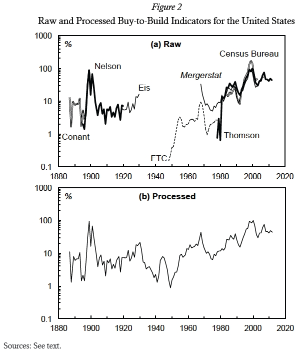
Constructing a series for the United States is more difficult because the data on mergers and acquisitions are less consistent and somewhat scarcer.[4] Seven sources can be identified:
1. Luther Conant’s (1901: 12) series for industrial companies during 1887-1900, covering those acquired worth over US$1 million, according to the total value of all their stock and bonds. Conant’s sources are unclear.
2. Ralph Nelson’s (1959: 145, 154, Tables B-3 & B-7) series for the manufacturing and mining sector during 1895-1920, based on reporting in the financial press, which tended to underreport smaller mergers.
3. Carl Eis’s (1969: 271, Table 1) series for industrial companies during 1919-30, covering consolidations worth at least US$1 million and acquisitions of US$100,000 or more, produced under the supervision of Nelson and using a similar methodology.
4. The Federal Trade Commission (FTC 1981: 104, Table 15) series for the manufacturing and mining sectors during 1948-79, in which the book value of the acquired firm’s assets were US$10 million or more. The US$10 million cut-off creates a major problem for the consistency of this series.
5. A series for 1968-2007 begun by W.T. Grimm & Co and subsequently published in Mergerstat Review (1991; 2008). The series covers all merger and acquisition announcements in the United States and by US companies abroad, including divestitures, and leveraged buy-outs. The series covers deals worth at least US$500,000 and is limited to only those mergers in which the value was made publicly available.[5]
6. A series published in the Statistical Abstract of the United States, covering the period 1984-2003 and including ‘mergers, acquisitions, acquisitions of partial interest that involve a 40% stake in the target or an investment of at least [US]$100 million, divestitures, and leveraged transactions that result in a change in ownership’ (US Bureau of the Census 1994: 551; also 2002: 493; 2004-05: 741). The source of these data was the Securities Data Company, which would later become Thomson Financial, and, as in the Mergerstat series, is limited to acquisitions in which the value was publicly announced.
7. Thomson Financial’s raw data on mergers and acquisitions, accessed through Thomson ONE Banker. All mergers and acquisitions in which the purchased company was located in the United States were included, while the total value of mergers was treated as the sum of all the announced values of each deal completed in each year.[6] Again, the major limitation is that it only includes deals in which the value was announced.
Once these series were compiled, each was divided by a series for gross fixed capital formation,[7] leading to six separate buy-to-build indicators. The results can be seen in part (a) of Figure 2.
Processing the various separate buy-to-build indicators was more complicated than in the case of Britain. Two series were used as bases. First, the indicator calculated from Nelson’s estimates for 1895-1920 was taken as a base, then extended to cover 1887-1930 using the Conant and Eis indicators, adjusted according to their average ratios with Nelson’s series during their overlapping periods. Second, the Thomson indicator was used for 1981-2012,[8] then extended back to 1968 using the Mergerstat Review series, again adjusted according to their average ratios with the Thomson indicator. The result was two series, covering 1887-1930 and 1968-2012 respectively. Interpolation to cover the gap between the two series was carried out in the same way as for Britain: exponential interpolation adjusted according to variations in a series of the number of mergers multiplied by a share price index,[9] divided by the series for gross fixed capital formation. The result was the processed series shown in part (b) of Figure 1.
Observations
Three main observations on the new series can be made:
1. The series for the United States differs considerably from that of Nitzan and Bichler (2009: 338, Figure 15.2), which appear to show a fairly continuous exponential trend from the late nineteenth century to the 2000s. By contrast, the new series is effectively trendless until after the Second World War, when a strong upward trend begins. This difference is principally because of an error in Nitzan and Bichler’s calculations, as they appear to have accidentally used figures for gross fixed capital formation in ‘constant’ 1929 prices up to 1928.[10] Prices in 1929 were notably inflated compared to the current prices of previous years, resulting in an artificially low buy-to-build indicator. Once the correct current prices are used, as in the new series, the buy-to-build indicator appears higher prior to 1929, doing away with the long-term upward trend. From this perspective, the Great Merger Wave of the 1890s appears truly great, as the buy-to-build indicator would not return to such levels until around the year 2000. Nitzan and Bichler’s (2009: 331) proposition that ‘[o]ver the longer haul, mergers and acquisitions tend to rise relative to green-field investment’ therefore becomes more problematic, with much depending on what qualifies as the ‘longer haul’.
2. There is a notable similarity between the British and US buy-to-build indicators, with both following similar patterns: essentially trendless up to the Second World War, with a strong upward trend thereafter. During 1887-2012 the Pearson correlation coefficient between the two series is 0.75, indicating a fairly close correlation. Capitalism, at least in the Anglo-Saxon countries, thus appears to have moved to similar rhythms on both sides of the Atlantic.
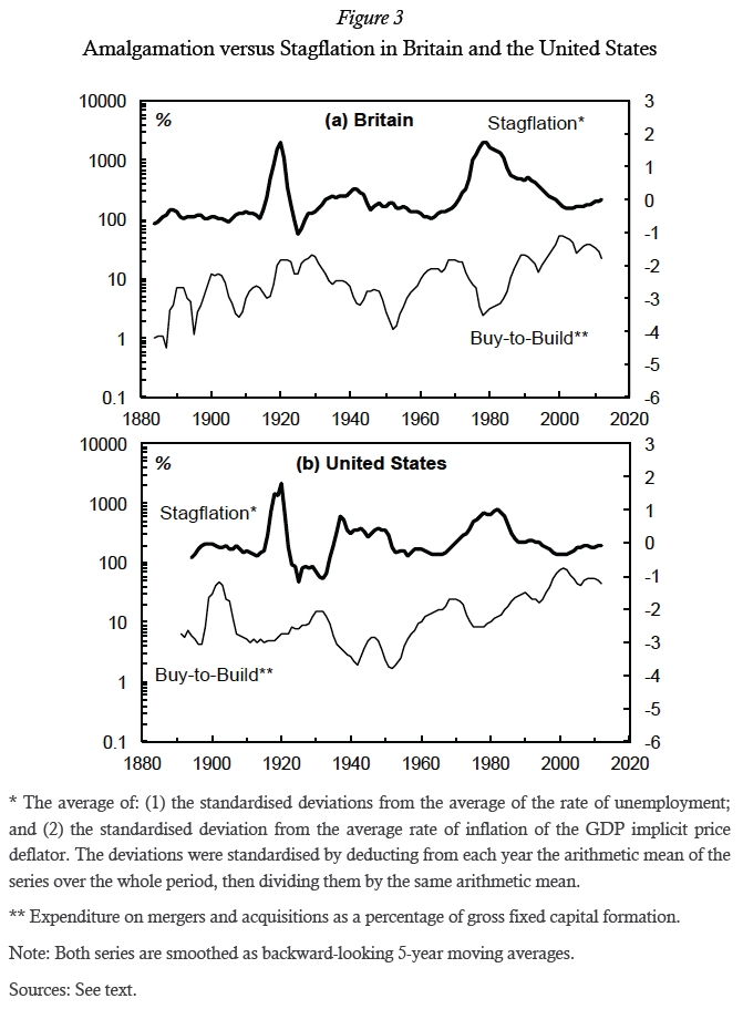
3. For both countries, the buy-to-build indicator has some correlation with Nitzan and Bichler’s (2009: 384, Figure 17.1) ‘Stagflation Index’, which they calculate as ‘the average of: (1) the standardized deviations from the average of the rate of unemployment; and (2) the standardized deviation from the average rate of inflation of the GDP implicit price deflator’. In Figure 3 the correlation can be seen in simple visual terms, as the Stagflation Index and the buy-to-build indicators tend to fluctuate in opposite directions.[11]
Endnotes
[*] Joseph Francis is a PhD candidate in Economic History at the London School of Economics (joefrancis505@yahoo.co.uk; http://www.joefrancis.info/). Shimshon Bichler teaches political economy at colleges and universities in Israel (tookie@barak.net.il; http://bnarchives.net). Jonathan Nitzan teaches political economy at York University in Toronto (nitzan@yorku.ca; http://bnarchives.net).
[**] This note draws on research that has been supported financially by the Economic and Social Research Council and the London School of Economics. Jonathan Nitzan and Roman Studer commented on an earlier version, although neither is responsible for any errors that remain. The workbook with the raw data and processing described is available at http://joefrancis.info/databases/Francis_buy_to_build.xlsx.
[1] Government statistics were used for 1948-2010 (ONS n.d.: Series NPQS), then extended back to 1880 using Charles Feinstein’s estimates (reproduced in Mitchell 1988: 831-35), adjusted them by the average ratio during the overlapping period.
[2] During 1919-39, Hannah gives low and high estimates. The average of the two was used.
[3] Hannah gives the number of mergers. The Actuaries General Share Price Index was taken from Global Financial Data (n.d.: Series GBAINDXW).
[4] For an overview, see Nelson (1959: Ch.2) and Golbe and White (1988: 267-75).
[5] The Mergerstat Review series has presumably been continued up to the present, although it proved impossible to check due to the cost of this publication.
[6] For 1981, for example, the precise search criteria were All Mergers & Acquisitions; Target Nation-United States of America; Date Effective/Unconditional-Between-01/01/1981 to 31/12/1981; Deal Basics Report.
[7] Bureau of Economic Analysis (BEA: n.d.: Table 1.1.5) data were used for gross fixed capital formation during 1929-2010, then extended backwards through ratio splicing with the estimates of Simon Kuznets (n.d.: Table T-8).
[8] The years 1976-80 appear to be very incomplete in the Thomson database, so they were not used.
[9] The number of mergers is was collated by the FTC (reproduced in Lamoreaux 2006: Series Ch422). The share price index is from Shiller (1989), updated at Shiller (n.d.).
[10] The series they reference is clearly in constant prices. See Nitzan and Bichler (2009: 360) and US Bureau of the Census (1975: I, 231, Series F105).
[11] For Britain, Feinstein’s unemployment rate was used for 1880-1947, then the National Insurance rate, then the ONS rate (from Mitchell 1988: 124; and ONS n.d.: Series MGSR); the inflation rate is based on the GDP deflator from Officer and Williamson (2013) for 1879-1948 and ONS (n.d.: Series IHYS) for 1948-2012. For the United States, the unemployment rate comes from US Bureau of the Census (1975: I, 135, Series D86; and n.d.); and the GDP deflator is from Johnson and Williamson (2013) for 1889-1929 and the BEA (n.d.) for 1929-2012.
References
BEA (Bureau of Economic Analysis) (n.d.) ‘National Income and Product Accounts’ (http://www.bea.gov/national/nipaweb/index.asp, accessed March 20th, 2013).
Conant, Jr., Luther (1901) ‘Industrial Consolidations in the United States’, Publications of the American Statistical Association, 7:53, 1-20.
Eis, Carl (1969) ‘The 1919-1930 Merger Movement in American Industry’, Journal of Law and Economics, 12:2, 267-96.
FTC (Federal Trade Commission) (1981) Statistical Report on Mergers and Acquisitions 1979.
Global Financial Data (n.d.), website, (https://www.globalfinancialdata.com, accessed March 19th, 2013).
Golbe, Devra L. and Lawrence J. White, ‘A Time-Series Analysis of Mergers and Acquisitions in the U.S. Economy’, in Alan J. Auerbach (ed.) (1988) Corporate Takeovers: Causes and Consequences (Chicago, IL: Univ. of Chicago), 265-310.
Hannah, Leslie (1983) The Rise of the Corporate Economy (2nd ed., London: Methuen).
Johnston, Louis and Samuel H. Williamson (2013) ‘What Was the U.S. GDP Then?’ (http://www.measuringworth.com/usgdp, accessed March 30th, 2013).
Kuznets, Simon (n.d.) ‘Annual Estimates, 1869-1955’, mimeo.
Lamoreaux, Naomi R. (2006) ‘Mergers, Acquisitions, and Joint Ventures: Number and Assets: 1919-1979’, in Carter, Susan B., Scott Sigmund Gartner, Michael R. Haines, Alan L. Olmstead, Richard Sutch and Gavin Wright (eds.) (2010) Historical Statistics of the United States: Millennial Edition (Cambridge Univ. Press, on-line: http://hsus.cambridge.org/HSUSWeb, accessed May 12th, 2011).
Mergerstat Review (1991) ‘Twenty-Five Year Satistical [sic] Review’, through LexisNexis (http://www.lexisnexis.com, accessed May 4th, 2011).
---. (2008) ‘Part Five Historical Review: Twenty-Five Year Statistical Review’, through LexisNexis (http://www.lexisnexis.com, accessed May 4th, 2011).
Mitchell, B.R. (1988) British Historical Statistics (Cambridge: Cambridge Univ. Press).
Nelson, Ralph L. (1959) Merger Movements in American Industry 1895-1956 (Princeton, NJ: Princeton Univ. Press).
Nitzan, Jonathan and Shimshon Bichler (2009) Capital as Power: A Study in Order and Creorder (London: Routledge).
---. (2002) The Global Political Economy of Israel (London: Pluto Press).
Officer, Lawrence H. and Samuel H. Williamson (2013) ‘What Was the U.K. GDP Then?’ (http://www.measuringworth.com/ukgdp, accessed March 20th, 2013).
ONS (Office for National Statistics) (n.d.), website, (http://www.statistics.gov.uk, accessed March 20th, 2013).
Shiller, Robert J. (1989) Market Volatility, Cambridge, MA: MIT Press.
---. (n.d.), website, (http://www.econ.yale.edu/~shiller/data.htm, accessed 14 October 2011)
Thomson Financial (n.d.), through Thomson ONE Banker, website, (http://banker.thomsonib.com, accessed March 19th, 2013).
US Bureau of the Census (1975) Historical Statistics of the United States: Colonial Times to 1870 (2 vols., Washington, D.C.: US Government Printing Office).
---. (various years), Statistical Abstract of the United States.
---. (n.d.), website, (http://www.census.gov, accessed March 20th, 2013).
Francis’ Buy-to-Build Estimates for Britain and the United States: A Comment
Shimshon Bichler and Jonathan Nitzan
Jerusalem and Montreal, April 2013
Francis’ new estimates of the buy-to-build indicator for the United States and Britain offer a welcome correction and addition to the U.S. numbers that we first presented in 1999 and later updated.[1] The three figures in this Comment elaborate on Francis’ findings.
Figure 1 plots the U.S. buy-to-build indicator estimated by Francis, along with our original numbers. The two series are tightly correlated, with a Pearson correlation coefficient of 0.87 for 1895‑2007. Francis notes that his U.S. series reveals the existence of two distinct sub-periods: (1) the era till the 1940s, during which the indicator was trendless; and (2) the postwar era, in which its trend was positive. This attempt to identify sub-periods is valid and potentially useful. In fact, his conclusion could have been drawn from our original estimates as well.
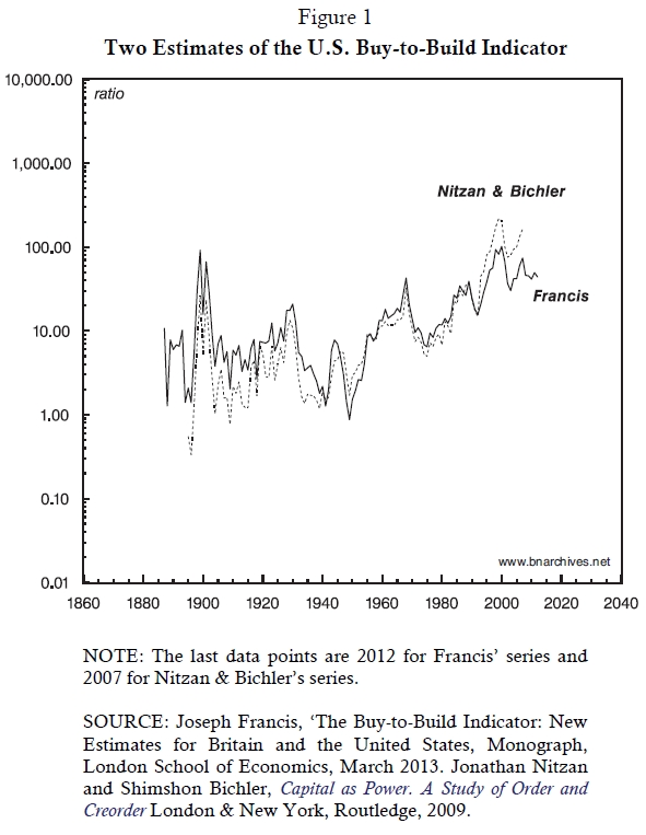
However, in and of itself, the identification of these two sub-periods does not seem to invalidate our original, broader claim; namely, that over the longer haul, the buy-to-build ratio tends to rise.
Both series in Figure 1 show four ‘high points’: (1) the peak of the ‘monopoly wave’ in 1899‑1901; (2) the peak of the ‘oligopoly wave’ in 1929‑30; (3) the peak of the ‘conglomerate wave’ in 1968; and (4) the peak of the ‘global wave’ in 1999-2000. Furthermore, with the exception of the second peak, each ‘high point’ is higher than the previous one – and that relationship, too, holds for both series.
So the key issue is the exceptionally high value of the 1899-1901 peak: does this high value invalidate our claim that the series as whole trends upward?
In our opinion, the answer is no.
The buy-to-build indicator is not like the seemingly eternal business cycle: it has a definite – and fairly recent – starting point. It acquired a positive value probably sometime in the 1870s or early 1880s, when mergers and acquisitions first emerged as a meaningful phenomenon together with the modern corporation and the associated market for corporate equities and bonds. Prior to that point, when there was little to acquire or merge with, the buy-to-build indicator had no clear meaning.
Now, note that Francis’ series begins not in the 1860s or the 1870s, but in the late 1880s, when the value of the buy-to-build ratio was already around 10. Unfortunately, there are no prior data on mergers and acquisitions, so the value of the indicator for earlier years remains known. But we can be pretty certain that during the preceding period the indicator was significantly lower, and that, at some point, it was close to or equal to zero. If we were to prefix Francis’ series with these unknown yet surely smaller numbers, the long-term trend of the full series would have been visibly positive – even with the ‘trendless’ sub-period of 1880-1940.
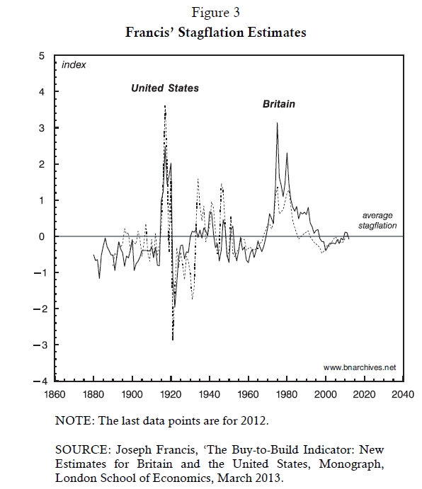
Figure 2 compares Francis’ buy-to-build indicators for the United States and Britain. The long-term trends of the two series are positive and very similar: the annual growth rate of the trend line is 1.8 per cent for the United States and 1.7 per cent for Britain. The two series also move in tandem, with a Pearson correlation coefficient of 0.73 for 1887-2012. A similar picture emerges from Figure 3, which plots Francis’ stagflation indicators for the two countries. Here, too, there is a tight correlation – 0.69 for 1890-2012. (Note that the stagflation indicator measures deviations from trend, so a value of zero represents the average rate of stagflation for the period.[2])
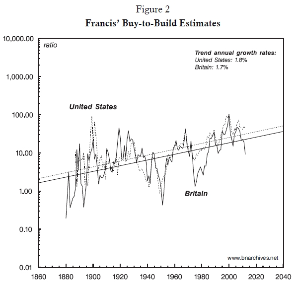
The co-movement and similar trends of the buy-to-build and stagflation indicators in the two countries are significant. They corroborate our suggestion that, over time, the global spread of differential accumulation helps synchronize the breadth-depth cycles across different countries.[3] The capital-market integration between the United States and Britain began in the middle of the nineteenth century, and that early start may explain why their breadth-depth cycles already moved in tandem at the turn of the twentieth century.
Endnotes
[1] The estimates were first given in Jonathan Nitzan, ‘Will the Global Merger Boom end in Global Stagflation? Differential Accumulation and the Pendulum of “Breadth” and “Depth”’, Paper read at International Studies Association Meetings, at Washington D.C., 1999. The most recent update is in Jonathan Nitzan and Shimshon Bichler, Capital as Power. A Study of Order and Creorder. RIPE Series in Global Political Economy. New York and London: Routledge, 2009.
[2] Jonathan Nitzan, ‘Regimes of Differential Accumulation: Mergers, Stagflation and the Logic of Globalization’, Review of International Political Economy 8 (2): Section 9; Jonathan Nitzan and Shimshon Bichler, The Global Political Economy of Israel, London: Pluto Press, 2002, pp. 72‑3.
[3] Jonathan Nitzan and Shimshon Bichler, The Global Political Economy of Israel, London: Pluto Press, 2002, pp. 47‑8.