Working Papers on Capital as Power, No. 2021/03, March 2021
The 1-2-3 Toolbox of Mainstream Economics: Promising Everything, Delivering Nothing
Shimshon Bichler and Jonathan Nitzan [1]
Jerusalem and Montreal
March 2021
![]()
bnarchives.net / Creative Commons (CC BY-NC-ND 4.0)
Preamble
We write this essay for both lay readers and scientists, though mainstream economists are welcome to enjoy it too. Our subject is the basic toolbox of mainstream economics. The most important tools in this box are demand, supply and equilibrium. All mainstream economists – as well as many heterodox ones – use these tools, pretty much all the time. They are essential. Without them, the entire discipline collapses. But in our view, these are not scientific tools. Economists manipulate them on paper with impeccable success (at least in their own opinion). But the manipulations are entirely imaginary. Contrary to what economists tell us, demand, supply and equilibrium do not carry over to the actual world: they cannot be empirically identified; they cannot be observed, directly or indirectly; and they certainly cannot be objectively measured. And this is a problem because science without objective empirical tools is hardly science at all.
1. Introduction
Our purpose in this paper is not to criticize demand, supply and equilibrium as such, but to show that, right or wrong, these tools do not translate into actual science. [2]
We begin in Section 2 with what we call the 1‑2‑3 toolbox of mainstream economics. Mainstream economists claim that the key tools in this box – namely, demand, supply and equilibrium – explain virtually any and every market. We argue they do not. In Section 3, we illustrate how in practice these tools produce baffling if not contradictory results and suggest they merit closer inspection. In Sections 4, 5 and 6 we offer a clean-slate outline of demand, supply and equilibrium analysis, show the price and quantity history of the U.S. shoe market, and illustrate how mainstream economists would use their 1‑2‑3 toolbox to explain it. Their explanation, though, is deeply problematic, and for the simplest of reasons: nobody, including economists, has any idea what demand, supply and equilibrium look like!
As we explain in Section 7 and 8, the demand and supply curves express the intentions of buyers and sellers, and these intentions are unknowable to outsiders (and sometimes even to those who supposedly possess them). In practice, the best economists can do is estimate demand and supply indirectly – and that does not work either. The first method, which we examine in Section 8, is to interview buyers and sellers. On the face of it, this method might seem sensible, but a deeper look shows its results are impossible to assess and often nonsensical. The second method is to estimate demand and supply curves econometrically, based on actual price and quantity data. In Section 9 we show that this method too runs into the wall. Demand and supply regressions, no matter how fancy, are tautological: they assume what they seek to prove. And that is hardly the end of it. Econometric estimates are only as good as the econometric models they are based on, and, as we show in Sections 10 to 12, these models – and therefore the estimates they generate – are virtually all bad (though nobody can say how bad, because the ‘true’ demand and supply curves, assuming they exist, are unknowable).
So, all in all, the 1‑2‑3 toolbox, even if perfectly effective on paper, is virtually useless in practice. It spews out tons of estimated coefficients, but these estimates have no demonstrable relation to the demand, supply and equilibrium they presumably represent. For all we know, these estimates are no more than ghosts in the minds of the estimators. And, as Section 13 illustrates, these ghost-like estimates often end up spread all over the place. On these counts, mainstream economics is not even close to being a science.
2. Demand, Supply and Equilibrium: The 1-2-3 Toolbox
The best place to start is at the beginning. Let’s look at how Gregory Mankiw, author of the best-selling introductory textbook, Principles of Economics (2018), introduces the subject to his first-year students. First, there is little pep talk:
When a cold snap hits Florida, the price of orange juice rises in supermarkets throughout the country. When the weather turns warm in New England every summer, the price of hotel rooms in the Caribbean plummets. When a war breaks out in the Middle East, the price of gasoline in the United States rises and the price of a used Cadillac falls. What do these events have in common? They all show the workings of supply and demand. (65)
‘Supply and demand’, says Mankiw, ‘are the two words economists use most often – and for good reason’:
Supply and demand are the forces that make market economies work. They determine the quantity of each good produced and the price at which it is sold. If you want to know how any event or policy will affect the economy, you must think first about how it will affect supply and demand. (65-66)
Next, he introduces the equilibrium of these two forces:
At the equilibrium price, the quantity of the good that buyers are willing and able to buy exactly balances the quantity that sellers are willing and able to sell. The equilibrium price is sometimes called the market-clearing price because, at this price, everyone in the market has been satisfied: Buyers have bought all they want to buy, and sellers have sold all they want to sell. (76-77)
And, then, when all is said and done, he delivers the ‘natural’ punchline:
The actions of buyers and sellers naturally move markets toward the equilibrium of supply and demand. (77)
Most economists will recognize this outline in their sleep: it is the neoclassical doctrine they teach and make their students rehearse. The uninitiated reader, though, may need a little explication, so here is a short outline.
The ideal neoclassical economy is a natural construct made up of numerous utility-maximizing agents. These agents are independent of each other, autonomous and rational. They have unlimited desires for hedonic pleasure, which they derive from consuming goods and services, but they have only limited means – or resources – to satisfy these desires. The difference between what they crave for and what they can afford generates ‘scarcity’. [3] Scarcity is inherent and permanent, so agents are compelled to produce, sell and buy more and more commodities without end. Their individual buying and selling desires-turned-intentions can be aggregated into market demand and supply curves. These curves interact in the market. Their interaction, mediated by the ‘invisible hand’ of pure competition, causes them to equilibrate. Equilibrium is a natural miracle that kills two birds in one stone: it generates the maximum attainable pleasure for market participants; and it answers the key question that economists never tire of asking: how much gets bought and sold, and at what price?
This is the pristine setup. The actual world, of course, is never as pure as mainstream economists would like it to be. So, when necessary, they tuck onto their ideal economy a whole slue of real-life distortions – from evil monopolies and perk-hungry labour unions, to arbitrary government regulations and unanticipated global shocks, to partial or wrong information, irrational calculations and capricious habits, among other ills. And yet – and this point is key – whatever the distorting menace, demand, supply and equilibrium can handle it. Or so we are told.
Mankiw’s 866-page doorstopper articulates this confidence with fervour. The book mentions the words demand, supply and equilibrium virtually on every leaf, and more than once. The most popular of the three is demand: it appears no less than 2,558 times – roughly 3 times per page. Supply is less frequent; it is mentioned only 1,985 times, or 2.3 times per page. The least common is equilibrium, which the book uses only 669 times, or 0.8 times per page.
These repetitions are typical. Table 1 compares the per-page occurrence of each term across five leading introductory textbooks: Bade and Parkin’s Foundations of Economics (2018), Case, Fair and Oster’s Principles of Economics (2012), Krugman and Wells’ Economics (2015), Mankiw’s Principles of Economics (2018) and Samuelson and Nordhaus’s Economics (2010).
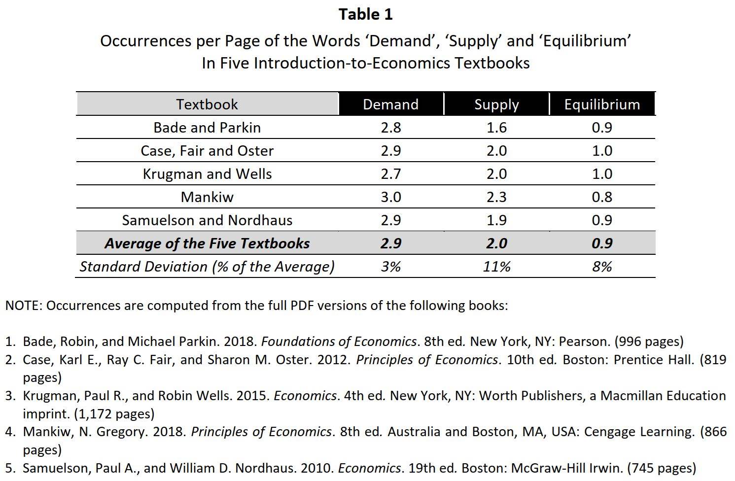
Remarkably, the per-page frequency of each word is almost identical across the five textbooks (note the tiny standard deviations in the bottom row).
If these frequencies are common to other textbooks, we can refer to demand, supply and equilibrium as the economists’ 1‑2‑3 toolbox. Equilibrium is the numeraire, with roughly one appearance per textbook page; supply is second in line with almost two; and demand leads the pack with nearly three.
Some may see these repetitions as a sign of confidence, but to us they look rather suspect. Unlike organized religion, science does not require reiterations. Instead, it lets logical argument and empirical evidence speak for themselves. So why don’t mainstream economists do the same? Why do they constantly repeat and praise the power of their 1‑2‑3 toolbox? Is there something wrong with this toolbox? Do they have something to hide?
3. Because and Despite in the Oil Market
In everyday discourse, the 1-2-3 toolbox is usually taken for granted. For most people, the ‘laws of demand and supply’ seem self-evident, even if they cannot clearly articulate them. They find it sensible that ‘scarce’ things rise in price while ‘abundant’ ones fall. And yet, in practice, few can pin down these seemingly self-evident principles. Table 2 illustrates this difficulty in the global oil market.
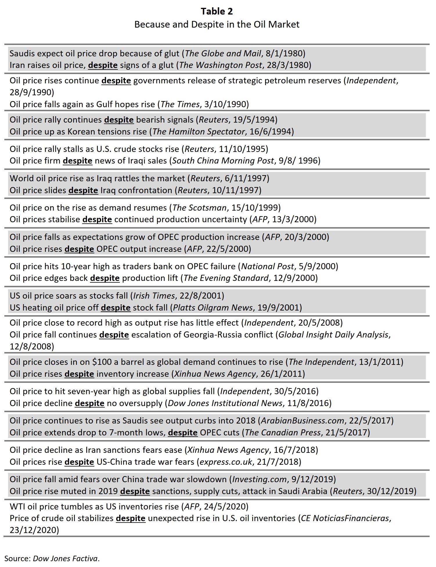
Oil is a highly standardized commodity whose price, many believe, moves up and down with its scarcity: when sellers want to sell less than buyers want to buy, scarcity increases and so does the price; and conversely, when sellers want to sell more than buyers wish to acquire, scarcity and price decline. But as Table 2 demonstrates, this common sense fails often.
The table pairs headlines that are less than a year apart. In each pair, one headline notes that the price of oil obeys the laws of demand and supply, while the other indicates it disobeys them. For example, the first headline might note that the price increased because of a glut, while the second, posted a couple of months later, might state that it fell despite the glut. Or one headline will note that the price fell because OPEC increased output, while the other will observe that it rose despite the higher output.
An economist might dismiss this table as a low-brow critique. After all, journalists seek drama, so they often cut corners, neglecting to mention other possible explanations. Nonetheless, the ease at which newspapers can use and abuse the same explanation suggests that maybe the 1-2-3 toolbox is not as omnipotent as economists want us to believe.
4. Demand, Supply and Equilibrium: The Essentials
To examine this possibility, let’s begin with the clean slate shown in Figure 1. This is probably the most famous graph in economics, and all economists know it by heart. But for our non-economist readers, we describe it briefly in the remainder of this section, just to make sure everyone is on the same page.
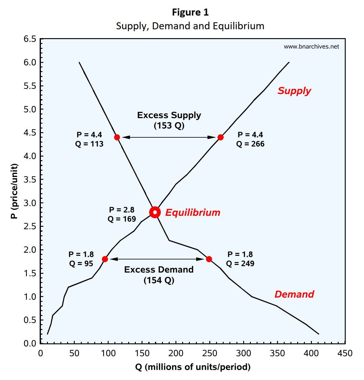
The graph pertains to a given commodity (such as shoes, carrots, or microchips), a particular market boundary (for instance, Esquerra de l’Eixample in Barcelona, the city of Beijing, or the United States as a whole) and a specific period (say as a day, a month, or a year).
The vertical axis shows the price of the commodity, P. This price is expressed in ‘real terms’, meaning it is measured not in nominal $, but relative to the average $ price of other commodities. To compute it, the economist will divide the commodity’s $ price by a $ price index of other commodities, so the result P is a pure number. [4] The horizontal axis shows the physical quantity of the commodity, Q – in this case, in millions of units – demanded and supplied during the period.
To illustrate with a concrete example, pretend that this chart shows the U.S. shoe market in 1995. The vertical axis will measure the ‘real’ price of U.S. shoes in 1995 – i.e., their $ price relative to the average $ price of all other U.S. consumer goods and services sold and bought in that year. The horizontal axis will show the overall number of shoes that were demanded and supplied in the United States in that same year.
Inside the chart we see two curves. The one going down from the top left to the bottom right is the demand curve. This line expresses the total desires of U.S. consumers to buy shoes at alternative prices, all else remaining the same.
The expression ‘all else remaining the same’ is here to remind us that the desires of consumers to buy the commodity in question – in this case, shoes – are determined not only by its relative price, but also by other factors. These factors include, among others, the number of consumers in the shoe market, their average income and the way in which this income is distributed among them, the relative prices of substitutes (like cloth to wrap your feet with?) and of complementary commodities (such as socks, shoelaces and shoe polish) and, of course, the very tastes of consumers (an umbrella term denoting the general structure of the demand curve for shoes as well as for all other commodities).
Now, just like the commodity’s price, these factors too tend to change. But here is the thing: according to economists, to isolate the specific effect of price on quantity demanded, we must assume – at least analytically – that these other factors are all unchanged. And since everything other than prices and quantities (and the odd parameter in a more complex inquiry) is assumed unaltered, this type of analysis can never be applied to actual time. It works only in hypothetical time. In actual time, price changes are always accompanied by changes in numerous other things. In hypothetical time, we can simply freeze all those other things. Economists call this synthetic type of analysis ‘comparative statics’.
The line rising from the bottom left to the top right is the supply curve. This line describes the desires of market sellers to sell the commodity at alternative prices – again, all else remaining the same. Here too, the desires to sell are affected by price as well as other determinants. These determinants include factors such as the number of potential shoe suppliers, the cost of the different factors of production (the machinery used up in production, labour, electricity, leather, nails, rubber, glue, etc.), the level of knowhow, the available fixed equipment, the relative prices of other commodities that shoe sellers can produce and/or sell (for example, leather coats, upholstery, plastic and rubber products) – and, finally, the way in which sellers mix these factors with profit considerations to generate their final selling intentions. And here too economists insist on comparative statics – in other words, on assuming, at least analytically, that all factors other than price remain fixed.
The intersection of demand and supply is the point of equilibrium. Economists like to think of this point as both desired and stable. It is desired because, when the price is 2.8 per unit, buyers can buy and sellers can sell exactly what they can afford and want to – namely 169 million units. And it is stable, first, because at this price there is no reason for either buyers or sellers to change their actions; and second, because if for some odd (read exogenous or irrational) reason the price deviates from equilibrium, market forces will immediately kick in, forcing it to converge back to that position.
For example, if the price happens to be 4.4 instead of 2.8, there will be an ‘excess supply’ of 153 million units. The excess occurs because, at that price, sellers will want to sell 266 million units – which is more than the 113 million units buyers will want to buy. Unlike equilibrium, excess supply is inherently unstable, or so we are told. Sellers, goes the argument, find themselves stuck with undesired inventories of shoes, so they start underbidding each other by lowering their price. As the price declines – assuming all else remains the same – buyers buy more and more. This process of shoe sellers lowering the price and shoe buyers increasing their quantity demanded will continue till the price reaches 2.8 per unit. No one knows how long this comparative-static process might take to complete. It can be instantaneous, stretch over ten years, or take any other period to terminate (all counted in units of hypothetical time). But once done, sellers and buyers will exchange exactly the quantities they wish to. And given that everyone is again satisfied, stability is happily restored.
The opposite situation is trigged by ‘excess demand’. For example, if the price happens to be only 1.8 per unit, buyers will want to buy 154 million shoes over and above what sellers would like to sell. Naturally, frustrated buyers who cannot buy the number of shoes they want at that price will compete by bidding it up. And as the price rises – all else remaining the same – sellers will supply more. The updrift will continue – again, nobody knows for how long – till the price of shoes reaches 2.8 per unit. At that point agents will again be as happy as they can be given the circumstances, and equilibrium will be safely reinstated.
Now, so far, we looked at how demand, supply and equilibrium determine a specific combination of price and quantity. But what causes prices and quantities to change? Here too the answer comes right out of the 1‑2‑3 toolbox – though this time the explanation is a bit different. Previously, we assumed that ‘all other conditions’ – from tastes, to the prices of other commodities, to incomes, distribution, cost and technology, etc. – remain fixed so that demand, supply and equilibrium stay put. But when one or more of these ‘other conditions’ varies, the result is that demand, supply or both shift and the point of equilibrium changes.
According to mainstream economists, the general principles here – which they label the ‘laws of supply and demand’ – are simple and elegant. When the demand curve shifts up or down along a fixed upward-slopping supply curve, quantity and price will move in the same direction – either up or down. Conversely, when the supply curve shifts either up and to the left or down and to right along a fixed downward-slopping demand curve, quantity and price will change in opposite directions – with one going up and the other down. And when both supply and demand shift, the movements of price and quantity will depend on the relative extent to which the two curves change. And that is pretty much all there is to it.
Neoclassicists celebrate this theoretical parsimony. Markets, they point out, are incredibly complex, yet much of this complexity can be sorted out with their simple 1‑2‑3 toolbox. No wonder this box is the Holly Grail of economics. With just three tools – demand, supply and equilibrium – it determines the quantities of sales, purchases and prices, along with plenty in-between. It can explain – with variations, modifications and distortions if necessary – the prices and quantities of every commodity, in every period, in every society. There is virtually no market it cannot account for.
There is only one little caveat. The 1‑2‑3 toolbox works only on paper. In practice, it accounts for virtually nothing.
5. The U.S. Market for Shoes
To see why, consider Figure 2. The chart shows the average annual ‘real’ prices and quantities of shoes in the United States from 1959 to 2020. The horizontal, quantity axis depicts ‘real’ consumer expenditures on shoes – i.e., dollar spending corrected for changes in shoe prices. This is how economists approximate aggregate quantities. The vertical axis shows the ‘real’ (read relative) price of shoes – namely, the price index for shoes divided by the price index for all consumer expenditures. Both magnitudes are normalized with 1959=100 (meaning that the price and quantity series are each divided by their respective magnitudes in 1959 and multiplied by 100).
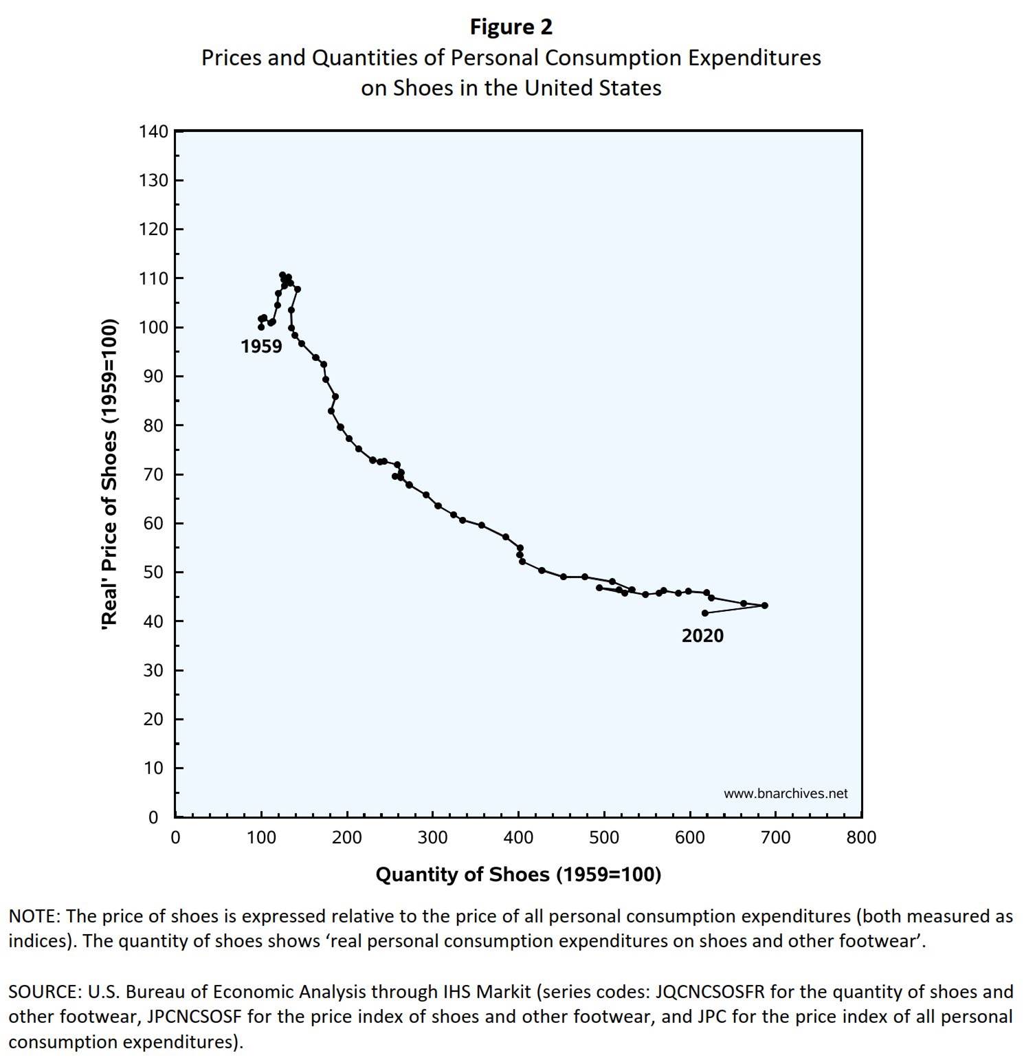
Now, the shoe market is not exactly the incarnation of ‘perfect competition’. The sell side, particularly the sport-shoe segment, is dominated by giants such as Nike, Adidas, New Balance, Asics and Kering (Puma). On the buy side there are many millions of buyers – but then, advertisement and other forms of conditioning serve to distort their ‘information’ and mess up their ‘sovereignty’ and ‘rationality’. There is also ‘government intervention’ in the form of regulation, taxation, tariffs, quotas and other chronic ills. But, for argument’s sake, let us ignore these minor glitches and assume that this market is purely competitive to the letter.
With this assumption in mind, what should we make of the time series shown in the chart? We can see that the quantities of shoe sold and bought in the United States have grown over time (indicated by the annual observations drifting to the right). We can also see that their ‘real’ prices relative to other consumer commodities have declined (shown by the observations edging downward). But what caused these long-term movements?
6. The 1-2-3 Toolbox in Action
The standard economic explanation is offered in Figure 3. As Figure 2, this chart too shows the prices and quantities in the U.S. shoe market for 1959-2020. But here we do more: we use the 1-2-3 toolbox to explain why these prices and quantities have changed. [5]
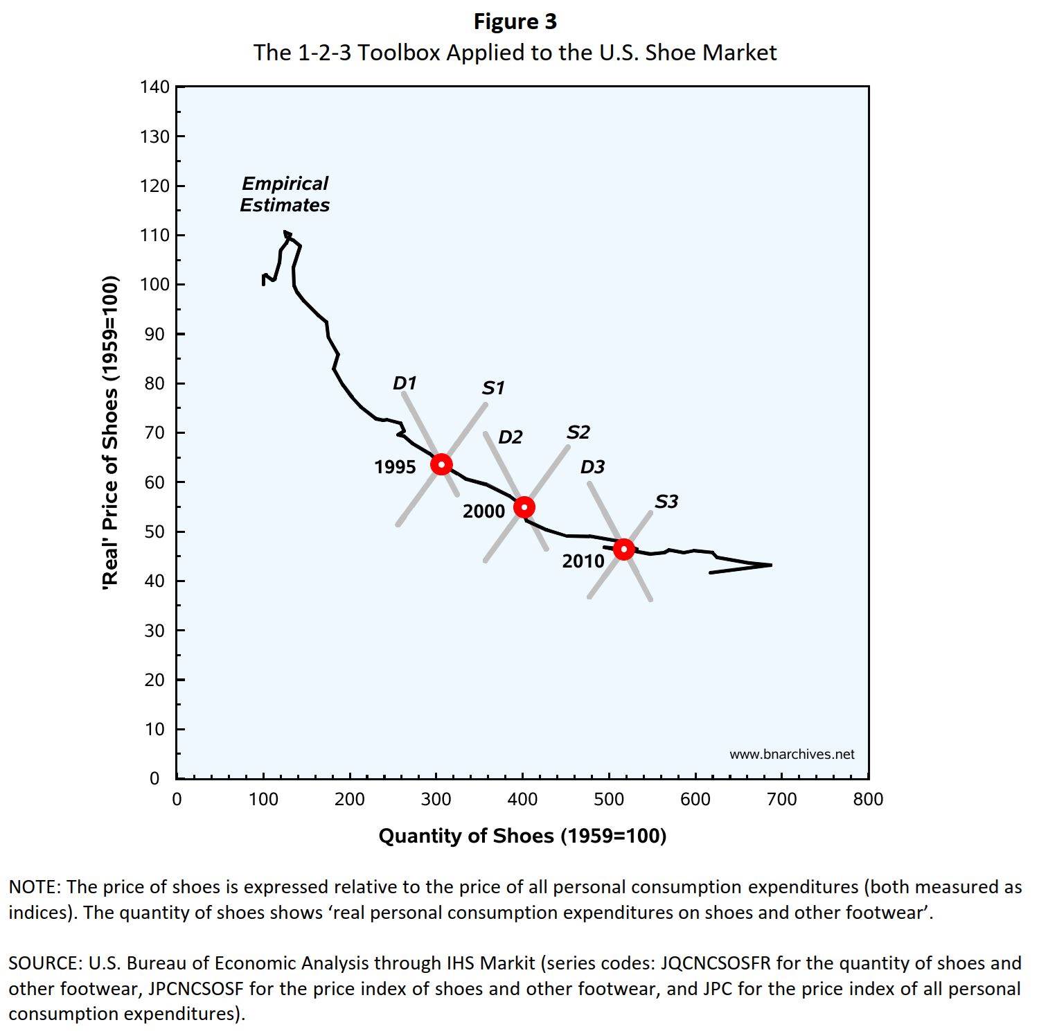
According to this explanation, each annual observation is a point of equilibrium between demand and supply. We illustrate this claim for three different years: 1995, 2000 and 2010. In 1995, the equilibrium was determined by the intersection between the demand curve D1 and the supply curve S1. During that year, ‘all else’ supposedly remained the same, so equilibrium stood still. In time, though, the ‘all else’ factors changed, and by 2000 these changes caused demand and supply to shift to new positions, indicated by D2 and S2, respectively. The empirical observation for 2000 emerged from the equilibrium of these new curves. And the same happened in subsequent years. Conditions continued to change, and the curves shifted with them. In 2010, demand and supply moved to D3 and S3, intersecting in yet another equilibrium – which, as you correctly guessed, produced the observed price and quantity for that year.
Since the explanation is general, it applies to every observation in the 1959-2020 series: as conditions and tastes changed, demand and supply shifted; with these shifts, each new equilibrium gave rise to a new empirical observation; and when we connect the dots, we get the entire time series. And this simple logic is by no means restricted to the U.S. shoe market of 1959‑2020. It can explain the market for any commodity, anywhere, anytime. It is universal. The only question is whether there is any science to it.
7. Where Do Demand and Supply Come From?
The title of this section may sound ironic, but the question is genuine. Note that, in simulating the neoclassical explanation, we drew each pair of demand and supply curves so it intersected exactly at the designated observation. But how did we know what these curves looked like and that they indeed equilibrated at those designated points?
The answer is we didn’t. Just like the neoclassicists, we have no idea what actual demand and supply curves look like. Just like the neoclassicists, we simply plotted them so that they intersected in the observations for 1995, 2000 and 2010. And like the neoclassicists, we did so because these intersections are consistent with the neoclassical doctrine.
But since our curves are imaginary, our explanation is irrefutable. We could have achieved the exact same accuracy – and irrefutability – by drawing imaginary cosmic rays through these observations, or by attributing their specific locations to the will of God.
When neoclassicists say that the time series in Figure 3 is the consequence of a rolling equilibrium between shifting demand and supply curves, they make a theoretical proposition. To assess this proposition scientifically, though, they must contrast it with actual data. Specifically, they must plot the actual demand and supply curves, show the way in which these actual curves shifted over time, demonstrate the exact points where they intersected, and compare these intersections with the time series shown in the figure. The problem is that none of these things can be done.
The five introductory textbooks listed in Table 1 offer no help in this matter. In fact, they skip it altogether. Their combined 4,600 pages mention demand, supply and equilibrium roughly 26,000 times, and they embellish these repetitions with thousands of multicolour pictures, tables and graphs. Yet none of these tomes provides a single picture, table or graph of an actual demand curve, supply curve, or equilibrium. Not even one! They also make no mention of how actual demand and supply curves can be estimated to start with. Lastly and most importantly, they fail to indicate that, for demand, supply and equilibrium to be scientifically useful, they must exist in the actual world and be known to economists. Perhaps the authors of these textbooks feel that these issues are better left to second-tier courses in ‘managerial economics’, where practical training and endless drill crush the remaining critical faculties of their fall-in-line students. [6]
8. What Can Economists Learn from Interviewing Agents?
So how can we find out what actual demand, supply and equilibrium look like? To reiterate, what we look for are desires. In their pristine incarnation, supply and demand curves represent the resource-constrained desires of fully autonomous, well-informed and totally rational utility-maximizing agents to buy and sell the commodity at alternative prices in a given market during a particular period of time, all else being the same.
Strictly speaking, the only way to know these desires – and the market demand and supply curves they give rise to – is to have direct access to the mind of each actor, find out their preferences and sum them up. [7] In the late nineteenth century, some economists fantasized having a ‘hedonimeter’ – a contraption that would measure these preferences directly from the agent’s mind or body. [8] So far, these fantasies have not materialized, and until they do, the only alternative is to ask the agents and hope they’ll answer honestly and accurately.
This alternative, though, is fraught with difficulties. To start with, markets can be very big. In the case of the U.S. shoe market, for example, we would have to ask hundreds of millions of buyers as well as hundreds or thousands of producers and retailers – and we would have to do so again and again every time preferences or market conditions change (which can be every month, every week, or even every day). Obviously, this is impractical even for a single commodity like shoes and inconceivable if we need to do the same for every commodity.
So how about interviewing only a small sample? Companies and economists conduct such interviews regularly, and assuming their samples represent their respective populations correctly, these interviews can be used to specify broader market demand and supply curves.
Or can they?
We admit having no idea how many such interviews have been conducted. But let us err on the upside and guess that, over the past century, an average of one million have been made annually around the world. Our guess implies that, in the last one hundred years, economists accumulated raw material for specifying as many as 108 actual demand and supply curves.
This number may look very large, but compared to the total number of demand and supply curves out there it is rather miniscule. To see how small, consider the following equation for computing the total number of demand and supply curves:
![]()
The overall number of commodities can be guesstimated by using the North American Industrial Classification System (NAICS) and the North American Product Classification System (NAPCS). These systems use a 10-digit coding for commodity types that can be further extended to account for specific items. This coding can accommodate billions of different commodities, so its order of magnitude is equal to or greater than 109. Next, consider that these commodities are bought and sold in hundreds of thousands of different markets – from world and national markets, to regional markets, to city and special markets – and that each of these markets has its own curves. The total number of these markets might be in the order of 105 or more. Finally, because tastes and conditions change continuously, each commodity in any given market will have as many demand and supply curves as the number of tastes-conditions sets. And if tastes and conditions change daily, over a period of a century we will need to estimate each curve tens of thousands of times – so the order of magnitude in this rubric is 104. Multiplying these three orders of magnitudes gives us 1018 actual demand and supply curves (of course, this calculation assumes that demand and supply are ontological entities to start with).
So even if we were able to derive perfectly accurate demand and supply curves from every interview ever conducted during the past century, the proportion of these derived curves out of the total would be only 1/1010 – or 0.00000001%. And this proportion would remain very small even if we overestimated the number of existing demand and supply curve several orders of magnitudes. Empirically speaking, then, the 1-2-3 toolbox is almost entirely empty.
Of course, the fact that interview-based estimates account for only a tiny proportion of existing demand and supply curves does not disqualify the underlying method as such. The important question is whether the method itself is reliable. And the answer to this question is that nobody can tell.
The main reason for this inherent limbo is that interview-based demand and supply curves can never be assessed, let alone verified. Recall that demand and supply estimates denote intended purchases and sales at alternative prices, and yet only one of those intentions – namely, the intention to buy and sell at the prevailing market price – can ever be contrasted with actual market data. The remaining intentions – i.e., the entire demand and supply curves less one point – never get expressed in the market, so there is no way to contrast them with actual price and quantity observations. [9] In this sense, economists can never know whether to believe what buyers and sellers tell them. The demand and supply curves they construct – whether based on the entire population or only a small sample – can be spot on, pure rubbish, or something in between, yet there is no way to tell which one it is. And this inability to judge is only amplified when using samples, since the extent to which these samples represent the underlying population is also impossible to assess! [10]
And that is just for starters. Whether interviewing all agents or just a sample, economists need to formulate their questions accurately and clearly so that interviewees understand exactly what they are being asked, and this requirement too is rather taxing. In the case of the U.S. shoe market, for example, interviewers of buyers would need to specify all available shoe types, sizes and attributes (so agents know what is on offer) and remind their interviewed subjects that, in answering their questions, they must keep ‘all things other than price unchanged’. These specifications can easily fill hundreds of pages, making everyone’s head spin.
And that is just for shoes, which is a rather simple commodity. Imagine what it takes to specify the full attributes of commodities such as electronic gadgets, cars, houses and complex financial services. Note that the specification of all these other commodities – which could number in the billions – is relevant, indeed essential, for the shoe market. According to the neoclassicists, utility-maximizing agents determine their buying preferences jointly for all commodities, so not knowing the nature of all those other commodities will make utility-maximizing demand curves – including for shoes – impossible to specify.
Finally, economists need to assume – without ever knowing whether their assumption is right or wrong – that the interviewees answer honestly; that they indeed mean to follow their stated intention; and, most importantly, that they have clear buying intentions in the first place.
This last requirement may seem bizarre: is it not obvious that consumers have buying intentions? Well, as it turns out, generally they do not! To see why, try to recall the last time you answered – or even asked yourself – the question ‘how many shoes do I intend to buy or sell at alternative prices, all else remaining the same’? Probably never. And how often have you asked and answered this question with respect to other commodities? Moreover, when you buy or sell commodities, how often do you stick to your earlier intentions, assuming you had any? The simple fact is that most people never spend time conceiving all-else-being-the-same price lists, let alone think of how they will adjust their quantity demanded and supplied as prices go up and down those lists. In this sense, most people – sorry, most ‘agents’ – have little or no conception of their individual supply and demand. If asked, they will simply answer off the top of their head.
In fact, even die-hard, fully informed utility maximizing wannabees will find it difficult to form consistent buying and selling intentions. A carefully designed experiment by Reinhard Sipple showed that, once the number of commodities exceeds a handful, consumers who otherwise seem perfectly ‘rational’ violate the most basic assumptions of neoclassical utility theory. The reason: they simply lose track of the rising number of commodities and the exponential increase in possible consumption bundles. [11]
In sum, the neoclassicists’ claim that their 1‑2‑3 toolbox can explain any and every market in the world is somewhat of an empty boast. In practice, demand, supply and equilibrium do not – and cannot – explain any, let alone all, markets simply because they are unknown. They can be guessed through interviews – but interview-based curves are logically dubious, statistically inadequate and, most importantly, empirically unverifiable. In this sense, the 1-2-3 toolbox is not almost empty, it is entirely empty.
9. Can Demand and Supply Curves be Derived from and Explain Market Data?
Informed readers – particularly economists – are likely to deem our last claim both pompous and ignorant. Economists, statisticians and businesspeople, they will point out, have been busy estimating actual demand curves, supply curves and equilibrium for over a century now, and these estimates, they will add, have been based not on flimsy interviews, but on hard market data and state-of-the-art econometrics. Bichler and Nitzan, they will opine, are spreading fake news. The economist’s 1-2-3 toolbox is not empty at all. In fact, it is overflowing.
And this counterclaim is partly true. The literature that derives empirical demand and supply curves from actual market data is indeed voluminous. However – and here is the key point – there is no objective way to show the the estimates produced by this large literature, no matter how data-grounded and econometrically sophisticated, have anything to do with the actual market demand and supply curves (again, assuming these curves exist).
To explain this last claim, we need to distinguish intentions from actions. Market demand and supply curves express intentions. They quantify the desires of autonomous buyers to buy and sellers to sell the relevant commodity at alternative prices, all else remaining the same. By contrast, empirical demand and supply curves estimated from market data reflect action. They mirror actual buying and selling.
And here is the problem. Mainstream economists assume that market data represent equilibrated demand and supply curves. They then use market data to estimate these demand and supply curves. And finally, they use the estimated curves to explain the market data they come from. In short, they go in a circle.
To flesh out the circularity, recall that, in their textbooks, mainstream economists argue that the intentions-read-desires of buyers and sellers (demand and supply) explain their actions (buying and selling), and that these actions in turn drive market outcomes (prices and quantities). This process is shown in Sequence 1:

Yet, in deriving their market-based estimates they go in reverse. Sequence 2 below is identical to Sequence 1, with one exception: its arrows, instead of pointing right-ward, point leftward. When following Sequence 2, economists begin from market outcomes, argue that these outcomes are created by the actions of agents, and conclude that these actions therefore represent the agents’ intentions – i.e., their market demand and supply curves:

And here is where things fall apart. Economists are free to believe that both sequences are valid. But, because the second sequence assumes the first, it cannot be used to prove it. And yet that is precisely what mainstream economists do. They estimate demand and supply curves from market outcomes (Sequence 2) – and then use these derived demand and supply curves to explain the very market outcomes their estimates come from (Sequence 1). In other words, they substitute a tautology for proof. [12]
9. Regression in Action: Running on Empty
Since tautologies are always true, we expect them to be neat. But using market-based demand and supply curves to explain market data is anything but neat. In fact, it is rather messy.
The main reason for the mess is that econometrics is ill-suited for estimating processes that are unknowable, unstable and out of equilibrium. And since demand and supply curves denote desires that cannot be known, that change constantly, and that might not be acted upon, it is no wonder their estimation is fraught with difficulties. [13]
The basic model involves two regressions, one for the quantity demanded Qd, the other for the quantity supplied Qs:
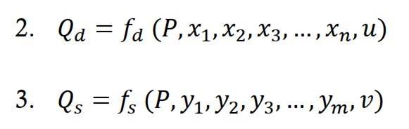
For those unschooled in econometrics, the glossary for the equations is as follows. In both equations, the elements on the right-hand side are said to determine those on the left. P is the observed market price of the commodity; the xi elements denote the n different conditions that determine the position of the demand curve as we saw in Section 4 and the yi elements are the m conditions that set the corresponding position of the supply curve; u and v are the equations’ error terms, representing the patternless white noise created by all excluded determinants (i.e., factors other than P and the xi and yi elements that do not appear in the equation but are impactful nonetheless); finally, fd and fs are the respective functional forms of the two regressions.
These regressions are supposed to help economists bypass the problem of comparative statics. As we saw in Section 4, comparative statics stipulates that in order to identify the relationships between price and the quantities demanded and supplied, we must assume that ‘all else remains the same’. This assumption is necessary because, unlike movements along the demand and supply curves which occur because of changing prices, shifts of the curves themselves are affected by changes in factors other than price (namely, the xi and yi elements in the two equations, as well as tastes for demand and profit considerations for supply). If these other factors are fixed, the curves stay put. If they change, the curves shift. Now, when economists engage in pure theory, they pretend that these other conditions are frozen and concentrate solely on how price changes affect the quantity demanded and supplied. But the actual world is dynamic, and since its conditions vary constantly, it is difficult to disentangle their effects from those of price proper.
This is where regression analysis comes to the rescue: it helps identify the unique impact of each of the right-hand factors on the left-hand variable of interest – in this case, the quantity demanded or supplied. And it does so by simulating the assumption of ‘all else being the same’ for every one of the right-hand side variables.
For example, applying Equation 2 to U.S. shoe-market data, the regression will estimate the unique effect on quantity demanded Qd of changes in price P, as well as of changes in each of the xi elements – including changes in the number of consumers, their average income, the distribution of their income, the prices of other commodities, etc.
But what appears neat on paper quickly gets scrambled in practice. The problem is that econometrics in general and regressions in particular are only as good as the assumptions on which they are based. If the assumptions are correct, so are the results. If they are wrong, the results are incorrect. And in the study of society – and of the economy generally and demand and supply particularly – the assumptions, and therefore the results, are virtually always wrong. Worse still, nobody can say exactly in what way they are wrong and by how much. [14]
Let us unzip these issues, beginning with the market’s demand and supply functions. As we saw in Section 8, economists cannot know these functions. Nonetheless, they specify them, and with great precision. Equations 2 and 3, for example, show very specific lists of determinants along with concrete functional forms. Do economists know that their specified equations are correct? Not in the least. They simply construct them as they see fit and estimate their coefficients.
Typically, they begin by choosing a functional form that suits their theoretical or practical fancy, populate it with a list of variables they like, input the necessary data, and, when everything is ready, hit the computer Enter key and examine the results. [15] The initial estimates tend to be all over the place and are seldom consistent with their specifier’s hypothesis and preferences. But not to worry. The next step is to add new variables and perhaps delete some of the existing ones, massage and transform the data, tweak the period of the study and rerun the regression. If the new results still fall short, the process begins anew. These cycles can be long and tedious, but with enough permutations they tend to improve the results, often markedly.
Occasionally, though, these re-adjustments don’t do the trick. And when that happens, the next step is to alter the equation’s functional form. For the lay reader, the functional form is the concrete mathematical structure of the equation. It determines whether the equation is linear or nonlinear, its particular shape, whether it contains lagged or multiplicative variables, the nature of the coefficient associated with each variable, whether these coefficients are fixed or varying (i.e., a function of other variables), the relationships between the different variables, the properties of the error term, and so on. In the case of the demand curve, this functional form represents the desires of consumers – i.e., the way in which they translate the values of the right-hand-side variables into buying intentions. In the case of the supply curve, it denotes how sellers weigh costs and profits in calculating their desires to sell.
Of course, since economists know virtually nothing about the actual desires of buyers and sellers, they cannot know the actual functional forms of their demand and supply curves. So, they specify these forms as they see fit – that is, in line with their theoretical inclinations, pragmatic dictates, or sheer fancy. And the fact that they can do so once, means that they do it again and again until the resulting estimates are deemed adequate.
Now, there is nothing inherently wrong in specifying and changing the variables and functional forms of these two equations, and in doing so repeatedly. After all, science involves plenty of trial and error by sleepwalking thinkers. But since the actual market demand and supply reflect desires that can be anything, and since the functional forms and determinants of these desires are forever unknowable, the econometric estimates – whether generated by a single computer run or after a thousand respecifications – will be correct only by an extremely improbable fluke. In other words, they will be wrong. Worse still, nobody can ever tell in what way they are wrong, in which direction, and by how much. The estimators, of course, will vehemently deny it, but these considerations suggest that their search for the elusive demand and supply curves is mostly running on empty.
10. Nonstationarity: When the Rules Change and Nobody Knows How
The final and perhaps most disturbing difficulties arise because the estimated processes are probably nonstationary and out of equilibrium. We look at these two difficulties in this and the next section.
Start from this fancy term, nonstationarity. Regressions, no matter how adaptive and dynamic, always end up imposing a fixed structure on reality. This imposition seems reasonable in the natural sciences, where it is common to assume that the ‘laws of nature’ do not change – or, in technical lingo, that they are stationary. Applying stationarity to the ‘laws of society’, though, seems rather presumptuous, if not silly. Society – including the economy – is not only in constant flux; it also alters its own governing principles. In other words, it is non-stationary. [16]
In fact, this nonstationarity lies at the very basis of neoclassical demand and supply. Mainstream economics glorify its autonomous agents. Agents are the basic building blocks of the economy, the sovereign masters whose rational choices generate the sacred ‘micro foundations’ of the entire discipline. But autonomy means freedom to change one’s own mind, alter one’s own desires, modify one’s own actions in relation to the broader world. And since neoclassicists insist that their agents are autonomous, it follows that demand and supply curves are doubly dynamic: not only do they shift because of external circumstances, they also self-transform their shape as agents alter their tastes and preferences.
In practical terms, this self-transformation means that the two curves can accommodate new variables and purge old ones, alter their coefficients and modify their overall mathematical structure, and that these changes will happen anytime agents change their mind. In short, demand and supply are inherently nonstationary – and to an unknowable degree to boot. And if, as the neoclassicists’ own theory implies, demand and supply can self-transform at any time, estimating them with fixed regressions – and arbitrary ones at that – is bound to generate even more meaningless results, if that were at all possible.
Neoclassical economists have addressed this nonstationarity mostly by assuming it away. On the demand side, economics Nobelist Milton Friedman conceded that wants ‘cannot be evaluated objectively’ but recommended that economists ‘take wants as fixed’ anyway. [17] George Stigler and Gary Becker, two other Nobelists, took a stronger, ontological stand, stipulating that tastes simply do not change (and that they are similar across agents). In their words: ‘tastes neither change capriciously nor differ importantly between people’. Just like the Rocky Mountains, they posit, actual tastes ‘are there, will be there next year, too, and are the same to all men’. [18]
On the supply side, the main solution is to enslave sellers to the fixed dictates of profit maximization. In this setup, autonomous sellers are reduced to mere algorithms, and since these algorithms simply translate objective costs to selling orders, nonstationarity disappears. The fact that, in practice, nobody knows what ‘maximum profit’ is, let alone how to achieve it, is usually neglected, or considered a non-issue.
To an outsider, insisting that demand and supply curves are stationary must sound featherbrained – if not deceitful, since it contradicts the agents’ presumed autonomy. But neoclassicists have no choice here. They must assume stationarity. Otherwise, they cannot even pretend to be doing science.
11. Out of Equilibrium: All Bets are Off
And then there is the possibility that the world is out of equilibrium. So far, we followed mainstream economists in assuming that buying and selling take place at equilibrium prices, and that actual prices and quantities trace the temporal shifting of demand, supply and their intersection (Figure 3).
But this assumption is invalid. In fact, it is invalid according to the neoclassicists’ own view. To see why, consider the four panels in Figure 4. Each panel reproduces the U.S. shoe market data from Figure 3. The panels also show different sets of hypothetical demand and supply curves for 1995. Panel 4-A represents the preferred neoclassical view, with the demand and supply curves intersecting at the market price and quantity for that year. But neoclassicists admit there are other possibilities.
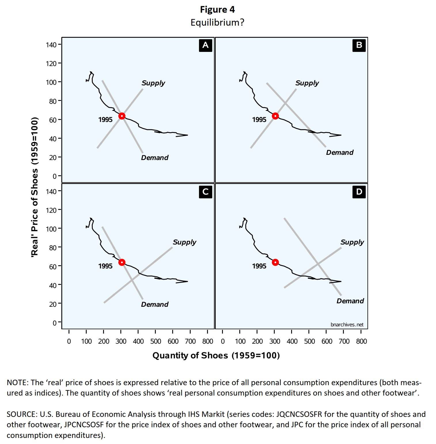
One such possibility is shown in Panel 4-B, where the 1995 price and quantity sit on the supply curve but not on the demand curve, creating excess demand. An opposite configuration is illustrated in Panel 4‑C, where the 1995 observation sits on the demand curve but not on the supply curve, leading to excess supply. And then there is Panel 4-D, which is doubly disturbing, because, here, the 1995 observation sits on neither curve. It just floats there, totally indifferent to the 1-2-3 toolbox.
Now, we have already seen that even if markets are always in demand-and-supply equilibrium, there is no way to empirically identify the actual demand and supply curves underlying this bliss. But what are economists to do when they face dis-equilibrium as illustrated in Panels 4B and 4C, or even non-equilibrium as shown in 4D?
Well, one popular solution is to assume that demand and supply discrepancies are eliminated instantaneously, so that markets are practically always in equilibrium. But this assumption is just as good as the opposite one, namely that markets never equilibrate. And the thing is that, in practice, no one can tell, simply because no one – including none of the profession’s 86 Nobelists – has ever managed to objectively identify an actual market equilibrium.
This inability means that, while econometricians think they trace actual demand and supply curves, or at least segments of these curves, in practice they are chasing ghosts. Without an objective yardstick, the likelihood that any specific market observation will sit on both the demand and supply curves (Panel 4A), or even on one of them (4B or 4C), is infinitely small. They most likely sit on neither (4D). And until we can tell which is which, all bets are off. Demand and supply cannot be estimated, even approximately.
12. An Example
These cumulative difficulties have consequences. Economists prefer to ignore these difficulties, so usually the consequences remain buried. But occasionally they bubble up to the surface, and in this section, we illustrate what happens when they do.
Our focus is the fish market. Fish is an important source of food with global annual sales in excess $160 billion, so there is plenty of interest in its demand curve. Also, according to many economists, the fish market is one of the few perfectly competitive markets left, so its demand curve should be relatively easy to estimates. Or so it seems.
Individual researchers are usually careful to report only consistent estimates and hide those that deviate too much from received convention. But they cannot control the estimates made by others, and when we compare various results, sometimes the differences are too large to ignore.
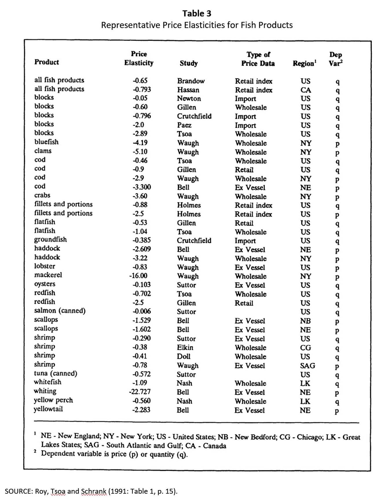
Table 3 illustrates this variance with estimates from 38 studies of the demand curve for fish conducted in different countries over more than half a century. The first column shows the type of fish, while the second gives the estimated price elasticity of demand.
For our lay reader, elasticity here measures the relative responsiveness of quantity demanded to a change in price (all else remaining the same), such that:
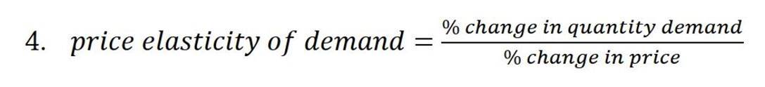
If the demand curve slopes downward, a given change in price will cause the quantity demanded to move in the opposite direction. And since the numerator and denominator in Equation 4 will have opposite signs, the elasticity will be negative.
The magnitude of the elasticity measures responsiveness. If it is smaller than –1, the relative change in quantity demanded is greater than the relative change in price, meaning the demand is elastic (i.e., responsive). For example, if a +5% change in price, all else remaining the same, leads to a –10% change in quantity demanded, the price elasticity of demand is –2. By contrast, if the elasticity is greater then –1, the relative change in quantity demanded is smaller than the relative change in price, so the demand is inelastic (irresponsive). For instance, a +5% change in price, all else remaining the same, leading to a –2.5% change in quantity demanded yields a price elasticity of demand of only –0.5.
Now, it would have been nice for economists if estimated demand elasticities for fish were broadly similar, but as Table 3 shows, their range is huge: from –0.006 for canned salmon (almost totally inelastic), to –22.7 for whiting (highly elastic).
The enormity of this range, including for the same type of fish, has not been lost on the article’s authors. This is their opening sentence: ‘What do statistical demand curves show?’ And their reply is brutal: ‘usually not as much as we would like, and frequently very little’ (Roy, Tsoa, and Schrank 1991: 13). You can almost sense the embarrassment behind the measured language:
The impetus for this study originated out of our concern with the inconclusive evidence on price elasticities of demand in a number of markets for primary commodities. A representative example, with which we are most familiar, is the market for fish products in the United States – a market described by one participant as ‘one of the last industries where demand and supply really plays a direct role’. Despite a number of demand studies on various segments of this market – to which we have made our own contribution – there is no consensus on the value of the price elasticity representative of this market. (14)
And this is from experts who have devoted a lifetime to the subject.
13. Summary
In this paper, we reviewed the scientific usefulness of the 1‑2‑3 toolbox of mainstream economics. The main tools in the box are demand, supply and equilibrium. Economists claim that these tools answer the two key questions of economics: how much gets exchanged and at what price. We argued they answer neither. Here is why:
1. According to mainstream economics, demand and supply represent the desires-read-intentions of buyers and sellers to buy and sell the commodity at alternative prices, all else remaining the same.
2. Nobody has direct access to these desires-read-intentions of buyers and sellers. In fact, most people never articulate their buying and selling desires in the first place, and the few who do quickly lose track of their preferences once the number of commodities exceeds a few dozens. In this sense, demand and supply curves might not even exist to start with.
3. Mainstream economists ignore these difficulties. They assume that demand and supply exist and insist they can be estimated, albeit indirectly, in two ways: (i) by interviewing agents about their buying and selling intentions; and (ii) by fitting econometric regression models to actual market data. Both methods have serious limitations.
4. Interview-based demand and supply curves are impossible to assess. Even if mainstream economics is correct, only a single point on the demand and supply curves ever gets expressed in the market. The rest are forever invisible. Consequently, there is no way to know – including after the fact – that the interviewees expressed their true buying and selling intentions (assuming they have such intentions to begin with).
5. Econometric-based estimates of demand and supply curves are tautological. Since these estimates assume that market data represent the intentions of buyers and sellers, they cannot be used to explain those intentions.
6. Econometric estimates of demand and supply are always wrong to an unknown degree. Valid regression estimates can be generated only by valid models, but in the case of demand and supply, the models are always invalid: (i) they are arbitrary and therefore almost certainly mis-specified; (ii) they impose a stationary structure on a self-transforming world; and (3) they assume, without a shred of evidence, that the world is in equilibrium. This triple mismatch means that even if demand and supply curves do exist, their estimates are nonetheless wrong – though nobody can ever say in what way and by how much.
These issues are yet to be addressed and resolved. In the meantime, mainstream economics remains a theology dressed as science. Like a well-organized religion, it promises everything and delivers nothing.
Endnotes
[1] Shimshon Bichler and Jonathan Nitzan teach political economy at colleges and universities in Israel and Canada, respectively. All their publications are available for free on The Bichler & Nitzan Archives (http://bnarchives.net). Work on this research note was partly supported by SSHRC.
[2] Perhaps the most accessible yet rigorous critique of mainstream economic theory is Keen (2011). For our own bit, see Nitzan and Bichler (2009: especially Chs. 5 and 8).
[3] We use scare quotes often in the paper, and for a reason: we find many concepts economists take for granted deeply problematic.
[4] For those in the know: the result is a pure number only if we can express all commodities in one universal unit, such as the ‘util’ they generate or the ‘SNALT’ (socially necessary abstract labour) they take to produce. There is no such universal unit, of course, but economists pretend it exists anyway.
[5] Incidentally, the U.S. shoe market was one of the first markets to which economists ‘fitted’ a statistical demand curve – sort of. See von Szeliski and Paradiso (1936).
[6] Managerial economics textbooks like Thomas and Maurice (2016), Samuel, Marks and Zagorsky (2021) and Baye and Prince (2021) teach ‘as-is’ practical techniques. They use the word ‘theory’ often, but mostly as an uncontested template of ‘how the world works’. Words such as ‘debate’, ‘critique’ and ‘disagreement’ are rarely if ever mentioned, and when they are mentioned, it is always in passing.
[7] Although this paper does not criticize neoclassical theory as such, it is worth noting that, contrary to what economists tell their first-year students, all-else-remaining-the-same market demand curves cannot be aggregated from individual demand curves. The reason is that a change in the price of the commodity – i.e., a movement along the individual demand curves – will alter the absolute and relative incomes of consumers. And since income and its distribution are two of those ‘all other things’ that supposedly remain the same, this movement on the demand curve will cause the curves themselves to shift, thus violating the assumption of comparative statics. For a clear explanation, see Keen (2011: Ch. 3).
[8] Francis Edgeworth (1881). See also David Colander (2007).
[9] In some markets, such as electricity, institutional sellers and buyers submit offers and bids, and when these offers and bids are ranked by price, they resemble upward-slopping supply and downward-sloping demand curves (see for example, Shah and Lisi 2019: Figure 2, p. 245). But this is an optical illusion. The observations on these curves are not the sum totals of the quantities supplied by all sellers and demanded by all buyers at each given price. Instead, each observation is a single offer or bid made by a different seller or buyer.
[10] Election pollsters can gauge how well their samples represent the population by comparing their prediction with the election outcome. Demand and supply curve pollsters, dealing with intentions that never get expressed in the market, do not have that luxury.
[11] Reinhard Sipple (1997). For a highly readable explanation, see Keen (2011: 67-72).
[12] Of course, economists might succeed in predicting out-of-sample prices and quantities. But even if they do, their success will not imply, let alone prove, that the estimated equations represent the underlying desires of buyers and sellers. It will simply mean that they found a good ‘fit’, and that the fit remained stable. The factors driving this fit could be many things other than the utility and profit-maximizing desires of autonomous agents.
[13] Some of these difficulties were pointed out, including by leading neoclassicists, almost a century ago – but generally to no avail. See for example Schultz (1923), Working (1927), Frisch (1933) and Stigler (1939).
[14] The debate over the adequacy of econometrics started with a famous exchange between John Maynard Keynes (1939) and Jan Tinbergen (1940) whose opposite arguments are yet to be reconciled. For an accessible assessment of the history, promises and travesties of econometrics, see Imad Moosa (2017, 2019).
[15] For fancy and largely inaccessible tracts on how to specify empirical demand and supply functions, see for example Pollak and Wales (1992), Fisher, Fleissing and Seletis (2001) and MacKay and Miller (2019).
[16] For a neat visual comparison between coefficient estimates in stationary physics and nostationary economics, see Moosa (2017: Figure 4.3, p. 81).
[18] Stigler and Becker (1977: 76).
References
Bade, Robin, and Michael Parkin. 2018. Foundations of Economics. 8th ed. New York, NY: Pearson.
Friedman, Milton. 1962. Price Theory. A Provisional Text. Chicago: Aldine Pub. Co.
Nitzan, Jonathan, and Shimshon Bichler. 2009. Capital as Power. A Study of Order and Creorder. RIPE Series in Global Political Economy. New York and London: Routledge.
Samuelson, Paul A., and William D. Nordhaus. 2010. Economics. 19th ed. Boston: McGraw-Hill Irwin.