Working Papers on Capital as Power, No. 2023/01, April 2023
Inflation as Redistribution: Creditors, Workers, Policymakers
Shimshon Bichler and Jonathan Nitzan [1]
Jerusalem and Montreal
April 2023
![]()
bnarchives.net / Creative Commons (CC BY-NC-ND 4.0)
A scientist is a mimosa when he himself has made a mistake, and a roaring lion when he discovers a mistake of others. (Albert Einstein, quoted in Calaprice 2011)
Abstract
This paper is part of a dialogue with Blair Fix on how inflation redistributes income between creditors and workers and the way in which monetary policy affects this process. In his 2023 paper, ‘Inflation! The Battle Between Creditors and Workers’, Fix shows, first, that the impact of U.S. inflation on creditor-worker distribution has been historically contingent (favouring workers during some periods and creditors in others); and second, that since the 1970s, Fed policy to combat inflation with higher interest rates boosted the yield of creditors relative to the wage rate of workers. Our own research suggests that these conclusions might be too general. We point out that creditors are not a monolithic class and that different types of creditors are affected differently, and often inversely, by the rate of interest. We illustrate that, contrary to bank depositors, bondholders tend to lose from inflation. And we show that monetary policy, at least in the United States, appears to follow rather than determine market yields. More generally, since most capitalists nowadays are lenders as well as borrowers, and given that ‘dominant capital’ profits from the full spectrum of investment instruments, we wonder if ‘creditors’ is still a useful category for analysing redistribution in general and inflationary redistribution in particular.
1. Introduction
The theory of capital as power (CasP) sees capitalism as a mode of power and capital as a form of power. Capitalists, the theory argues, seek to augment their relative power, and the extent to which they achieve this quest is quantified by the upward redistribution – or differential accumulation – of income and assets in their favour (Nitzan and Bichler 2009).
According to CasP, one of the key drivers of differential accumulation is inflation. The inflation process, we argue, is inherently redistributional, and this inherent feature, although seldom studied, is everywhere. Inflation redistributes income and assets between large and small firms, capitalists and workers, big landowners and small peasants, different sectors, various countries, private and governmental entities, etc.
The conventional creed rejects this view. In common economic parlance, inflation is conceived in the aggregate: it denotes a general rise in the prices of goods and services. In this sense, the very language of economics diverts our thinking away from redistribution. To illustrate, here is how two economic Nobelists define inflation in their introductory doorstopper (with our added italics):
Inflation occurs when the general level of prices is rising. Today, we calculate inflation by using price indexes—weighted averages of the prices of thousands of individual products. The consumer price index (CPI) measures the cost of a market basket of consumer goods and services relative to the cost of that bundle during a particular base year. The GDP deflator is the price of all of the different components of GDP. (Samuelson and Nordhaus 2010: 609)
Note Samuelson and Nordhaus’ repeated reference to aggregates – ‘general’, ‘average’, ‘basket’ and ‘all’. This aggregation serves to hide the underlying feature that matters the most – namely, that individual prices never change at the same rate. This is a simple but critical fact. It means that inflation transfers income from those who raise their prices by less to those who raise them by more. In other words, it means that inflation is always and everywhere redistributional.
What does ‘inflation as redistribution’ look like? Who are its winners and losers? Are they the same or different over time and across space? Is the redistributional process random or systematic? Is its impact small or large? Are its patterns stable or changing? While economists and popular commentators tend to conceive winners and losers in terms of ‘rich versus poor’, CasP sees this question as part of the much broader vista of power relations. How are social relations of power manifested through strategic sabotage and stagnation to fuel differential inflation and stagflation? How do differential inflation and stagflation restructure society and redistribute income and assets? Under what circumstances and to what extent does inflation as redistribution promote differential accumulation? ‘Rich versus poor’ is merely one aspect of these larger processes that create the order of – or creorder – the capitalist mode of power.
CasP researchers have tried to address some of these questions for different places (including Canada, Israel, Pakistan, South Africa, the United States and the world as a whole) and for various entities (such as capitalists and workers, large and small firms and various sectors). But their studies, being few and far between, have only scratched the surface of this crucial process. [2]
Inflation as redistribution is hard to study. The difficulty begins with the very measure of inflation. If Granny Smith apples cost $3.3/kg, up from $3 in the previous year, you know that the price changed by 10 per cent. But what about the price of ‘all apples’, or of ‘food in general’? Recall that inflation measures the price change not of one but of many commodities. So, what does it mean when the statisticians tell us that ‘food-price inflation’ this year was 15 per cent? If the statistical food basket in question remained unchanged, we could treat it as a composite commodity whose price increased by 15 per cent. But, in practice, the food basket – or any other commodity basket for that matter – never stays the same. It constantly changes – first, because sellers alter the qualities of the individual commodities they sell (the sausages are different, the cereals are modified, the cheese is altered); and second, because buyers change the relative quantities of the commodities they purchase (a new kind of TV dinner enters the basket, relatively more sausages are bought, relatively less cereals and beer are purchased). These modifications mean that, when we compare the price of a basket in period t to its price in period t-1, we are comparing the prices not of the same basket, but of two different baskets.
This
is a serious problem, but economists claim to have solved it. They do so in
three easy steps. First, they quantify the basket’s changing quality; second, they
use this measured quality to adjust the basket’s quantity; and finally, they
recalibrate the price change to the basket’s new size. To illustrate, if the basket’s
overall quality rose by 10 per cent, the economists would conclude that its quantity
is now 10 per cent greater. And if the basket is 10 per cent bigger, the
observed price increase represents a change in quantity as well as price.
Although the measured price is 15 per cent higher, the increase applies to a
basket whose quantity is now 10 per cent larger. The pure rate of inflation,
therefore, is not 15 per cent, but only 4.5 per cent = (1.15/1.1 – 1) ![]() 100.
100.
There is only one little difficulty: these adjustments are all arbitrary. To make them, economists must assume that actual markets are perfectly competitive; that prices correspond to the hedonic properties of commodity qualities; and that they, the economists, know how to quantify this correspondence and identify the equilibrium point at which it is manifested. Since these assumptions are invariably false (not to say fraudulent), the adjustments that rest on them are forever bogus and the inflation measures they yield are always inaccurate to an unknown extent (if not conceptually meaningless). [3]
Then, there is the void of absent prices. Statistical services group individual prices by commodity types – the price of energy, the price of pharmaceutical products, the price of entertainment, the price of financial services, etc. But when it comes to the distribution of income and assets, we need to know who sets what prices and who pays them, and this price information is seldom if ever available or even compiled.
While we might know the price index for software in general, we do not have separate price indices for Microsoft, Oracle and SAP products. We have price indices for military hardware, but not for the weapons sold specifically by Lockheed Martin, Raytheon and Boeing. We have wage indices for different types of workers, but not separate indicators for those working at Amazon, Google and Facebook. Similarly, we seldom know who pays what prices. While there are consumer baskets for different regions/commodity types, the data are rarely if ever grouped by the income levels of buyers (for example, there are no separate consumer-price indices by income deciles). And the smoke is even thicker when it comes to corporations, whose purchases and the prices they pay are deemed ‘proprietary’ and therefore kept undisclosed.
Finally, there is the much broader question of whether we should think of inflation as a stand-alone variable in the economist’s arsenal, or as a process that is deeply interlaced with and shapes the political-economic space. The former, conventional view sees various concepts and processes such as ‘technology’, ‘GDP’, ‘growth’, ‘income’, ‘government’, ‘capital’ and ‘inflation’ as distinct entities that interact with each other in an otherwise independent Newtonian space called ‘the market’. The latter view, which CasP prefers, is that the social space is not Newtonian, but Leibnitzian. It does not exist on its own, but rather is defined, bent and transformed by the entities that comprise it. Seen from this latter perspective, inflation is not separate from the strategic sabotage and stagnation that causes it or the constant redistribution of income and assets it engenders.
Taken together, these conceptual quandaries, missing data and the perception of inflation as part and parcel of the changing structure of society, make the study of inflationary redistribution truly daunting. To engage in such research, you must come up with thoughtful simplifications that do not sacrifice reality, create clever constructs and indices to transcend the vast voids of missing data and rethink the ways in which price changes creorder the very structure of society.
***
In this context, it is heart-warming to observe young researchers like Blair Fix taking the challenge head on. In a recent thought-provoking and meticulously researched paper series, Fix offers a biting critique of conventional theories of inflation and stagflation, presents an alternative research framework and provides new findings on inflationary redistribution. [4] But, as often happens with path-breaking forays into uncharted territory, his too brings to the fore new questions and difficulties worth exploring.
The purpose of our paper is to address some of these questions and difficulties. Our specific focus is Fix’s article, ‘Inflation! The Battle Between Creditors and Workers’ (2023d), in which he analyses the long-term relation between inflation and the distribution of income between U.S. creditors and workers. The study is novel – the subject of creditor-worker distribution has never been examined from a CasP perspective before – and it presents highly interesting findings and conclusions. But in our view, it conceives the redistribution process in question too generally. Specifically, it lumps together different creditors as if they share the same goal – the bond yield (a proxy for the rate of interest) – and in our opinion this lumping may be wrong. The bond yield (and the rate of interest more generally) may not be the goal of all creditors and generalizing it as such could render some of Fix’s conclusions incorrect.
We lay out our argument in steps. In the second section, we summarize Fix’s claims and main findings. In the third section, we differentiate between various types of creditors, identify the goal of each type and describe how each goal relates to the bond yield. Our fourth section focuses specifically on non-bearer (or tradeable) bonds, empirically examining the total income these bonds generate to their owners (capital gains and interest) and how this total income relates to their bond yield. The fifth section presents our own findings on the distribution of income between bondholders and wage earners. The sixth section studies how this distribution correlates with inflation. The seventh section uses a single dataset to systematically compare our own definitions, analysis and empirical findings to Fix’s. The eighth section deals with policymaking, examining whether it is the Federal Reserve Board (or Fed) that sets the U.S. rate of interest and in so doing affects the distribution of income, or whether the process is driven by capitalists who determine the U.S. bond-market yield, and the Fed simply parrots them. The nineth section closes with concluding thoughts.
2. Creditors versus Workers: Blair Fix’s Take
Fix begins by identifying the incomes of creditors and workers. Creditors receive interest payments, which he proxies by the annual per cent yield on long-term bonds (using an average of various bond instruments till 1960, spliced with government bonds thereafter). By contrast, workers earn wages, which he measures by the wage rate of unskilled workers.
Next, he quantifies the process of redistribution between creditors and workers in three steps, by (1) calculating the annual rate of change of bond yields (the income of creditors); (2) computing the annual rate of change of wages (the income of workers); and (3) subtracting the latter from the former. He dubs this difference between the two types of income growth the bond-wage growth gap.
Figure 4 of his paper, which we reproduce here, shows how this gap evolved from 1830 to the present. A positive reading in the figure means that the rate of return of creditors rises faster than that the income of workers (creditors win), whereas a negative reading implies that the income of workers rises faster than the rate of return of creditors (workers win). By inspecting these magnitudes, we can see who won and lost and by how much, as well as how the resulting redistribution evolved over time (most data are negative and the historical trend is downward, i.e., favouring workers at an increasing pace).
(Note that the bond-wage growth gap tells us about the relation between the incomes of the two groups, not the incomes themselves. In other words, the fact that creditors win relative to workers does not mean that their absolute rate of return rises; for example, both their rate of return and the income of workers could be falling, but if the rate for creditors falls more slowly than the wage rate, the bond-wage growth gap will still be positive.)
Finally, using the bond-wage growth gap, Fix assess how the redistribution of income between creditors and workers relates to inflation. To quantify this relation, he correlates the bond-wage growth gap with the rate of consumer-price inflation, using a moving, 30-year trailing correlation window. In this way, each annual reading indicates the correlation over the previous three decades, and the fact that the correlation window moves in annual increments allows us to assess how the redistributional effect of inflation changes over time. This moving correlation is depicted in Figure 5, which we reproduce from his paper.
When the correlation in Fix’s Figure 5 is positive, we know that in the previous 30 years inflation benefited creditors relative to workers (by helping them raise their bond yield faster than the wage rate). And, conversely, when the correlation is negative, it means that over the previous 30 years inflation helped workers raise their wage rate faster than creditors raised their yield.
And the historical pattern of this correlation is telling: rather than being either positive or negative, it oscillates. In some periods – notably, between the 1820s and 1850s, during the 1910s and since the late 1970s – the correlation was positive, meaning that, in those periods, inflation benefited creditors relative to workers, while in other periods – specifically, from 1860 to the 1900s and from 1910 till the late 1970s – the correlation was negative, suggesting that inflation favoured workers over creditors.
In other words, according to Fix’s analysis, the relation between U.S. inflation and creditor-worker redistribution is historically contingent. And that fact leads him to an interesting conclusion. He observes that, since the 1970s, mainstream economists have favoured ‘fighting’ inflation with higher interest rates and suggests that the fact that the U.S. Fed implemented this policy recipe shows the extent to which it has catered to creditors rather than workers. When inflation rises, the central bank fights it with higher interest rates, and the higher the rate of interest, the greater the benefit to creditors relative to workers (whose wages do not benefit from higher interest rates).
3. Who are the Creditors and What do They Want?
Fix’s research is analytically sharp, empirically meticulous and politically telling – yet, in our view, it tells only part of the story.
The main problem is the identity of creditors and the income – or yield – they are supposedly after. Fix correctly identifies creditors as ‘investors who earn interest’, including banks, credit card operations, bondholders and bank depositors, among others (Fix 2023d: Footnote 1). But then he singles out the goal of these creditors as the interest payments they receive – and in our opinion, this association is too general and often incorrect.
The difficulty here is twofold. First, the rate of interest can have different and possibly inverse effects on the income of any given creditor. For example, a rise in the rate of interest might cause the volume of lending by a creditor to shrink by even more, causing the overall amount of earned interest to contract. Or a falling rate of interest might reduce the lending income of a creditor but boost her equity portfolio by more, yielding a positive return altogether. These possibilities are difficult to investigate empirically, and we do not pursue them here.
The second obstacle is that creditors are not created equal: some benefit from a higher rate of interest; for some, the impact is uncertain; and for others higher rates might imply a loss. Let us consider these differences more closely.
The simplest case is creditors whose principal does not change. In this group we find bank depositors, whose accounts are non-tradeable and therefore have no floating ‘market price’. The value of such accounts – which represent the depositor’s principal – is always equal to the money balance they contain. Depositors earn an interest rate on these deposits, and that’s it. When the deposit rate rises, they gain; when it falls, they lose.
The same situation applies to buyers of bearer bonds (i.e., non-tradeable bills). They too benefit when the rate of interest rises and lose when it falls (though once they have acquired the bond, changes in the rate of interest no longer impact the income they receive from that bond). Fix’s focus on the rate of interest is adequate for this type of creditors.
But other creditors can have other goals in mind. Take banks. For them, the relevant yield is not the rate at which they lend. Instead, it is the difference – or net margin – between the interest rate they lend at and the interest rate they pay depositors. And as it turns out, this net margin shows no stable relation with the rate of interest (Ennis, Fessenden, and Walter 2016; Wheelock 2016). The same ambiguity applies to credit-card operations: their income, too, depends on the net margin between lending and borrowing rates – and that margin, again, has no obvious relation to the rate of interest (Adams, Bord, and Katcher 2022).
Owners
of non-bearer bonds – i.e., bonds that are bought and sold on the market – present
yet another case. If the annual ‘coupon’, or interest payment, on a U.S.
Treasury Bill is $60 and the bill is priced at $1,000 in the market, the yield is
6 per cent (= $60/$1,000 ![]() 100).
But the coupon payment is not the only income of a non-bearer bond holder.
[5]
100).
But the coupon payment is not the only income of a non-bearer bond holder.
[5]
Because
they are traded on the market, non-bearer bonds constantly change in price. If
the market price goes up (or down), the bond yield – i.e., the ratio
between the bond’s interest payment and market price – goes down (or up).
If the price in our example rises to $1,200, its yield drops to 5 per cent (= $60/$1200
![]() 100).
But this calculation is meaningful only to new bond buyers. To existing
bondholders, the income in this case is not $60, but $260: it comprises the
$60 coupon payment plus a $200 capital gain. For them, the yield is not 5 per
cent, but 26 per cent (= $260/$1,000
100).
But this calculation is meaningful only to new bond buyers. To existing
bondholders, the income in this case is not $60, but $260: it comprises the
$60 coupon payment plus a $200 capital gain. For them, the yield is not 5 per
cent, but 26 per cent (= $260/$1,000 ![]() ).
).
These differences make it difficult to lump all creditors together as if they share the same goal, and even more difficult to identify this goal as the rate of interest. While Fix’s analysis is applicable to the case of bank depositors and non-bearer bond holders, it is inapplicable and possibly misleading for other creditors such as financial institutions and non-bearer bond holders.
One last point. Fix’s measurement of creditor-worker redistribution – the bond-wage growth gap – denotes the difference between the rate of growth of the yield and the rate of growth of the wage rate. But these are not comparable income flows. Whereas the wage rate is counted in dollars per year, the yield is measured in per cent per year (interest payment relative to the extended credit), and so, strictly speaking, the difference between the rates of growth of these two magnitudes does not measure the redistribution of income between creditors and workers.
4. The Case of Bondholders
To resolve these issues, it is useful to (1) concentrate on a particular type of creditors; and (2) measure the income of such creditors in units comparable to those of the wage rate.
In what follows, we focus on bondholders – and specifically on holders of non-bearer bonds whose price varies on the bond market. The reason for this choice is threefold: first, in the United States – which Fix studies and so will we – bonds are a major form of credit (accounting for half of all outstanding debt, public and private); second, the analysis of these bonds is relatively straightforward; and third, Fix’s empirical research uses the bond yield, so our results can be compared to his. (From now on, and unless noted otherwise, we use ‘bonds’ and ‘bondholders’ to denote non-bearer bonds and their owners.)
Next, we measure the income of bondholders not by their per cent yield, but by the dollar sum of their capital gains (which can be positive or negative) and the interest payments they receive. This measure is directly comparable to the dollar wage rate of workers.
The combined dollar income of bondholders can be derived from the so-called total-return index, calculated by different data agencies. The agency calculating this index tracks the prevailing market price of the bond, adding onto it the periodic coupon payments, as if those payments are ‘reinvested’ in the same bond and therefore augment the sum owned by bondholders (though, in practice, bondholders may or may not follow this path). After the interest payments are (notionally) ‘reinvested’, the agency applies the next relative price change not to the previous market price of the bond, but to its coupon-augmented price. [6] In this way, the temporal evolution of the total-return index reflects both the appreciation/depreciation of the bond’s price as well as the compounded bondholders’ coupon income.
Figure 1 shows three indicators for 10-year U.S. government bonds, all smoothed as 10-year trailing averages. The dashed blue series plots the total-return index, while the solid blue series shows the dollar sum of capital gains and interest payments received by bondholders. The latter series is derived, for any given year, by subtracting from the total-return index of that year the total-return index of the previous one (both series are normalized with 1796=1.0 and shown against the left logarithmic scale). The hollow red series at the bottom of the chart depicts the per cent yield on those bonds, plotted against the right scale. [7]
As the figure makes clear, the dollar income of bondholders and their per cent yield are two different creatures: not only are they denominated in different units (dollars per year versus per cent per year), but they also move in different directions – the former trends up exponentially, the latter points sideways – and they display no clear correlation.
5. Bondholders versus Workers
The next step, shown in Figure 2, is to quantify the process of redistribution between bondholders and workers according to our own definitions.
The top panel of the figure compares the incomes of bondholders and wage earners, with both series smoothed as 10-year trailing averages and normalized with 1799=1.0. The bondholder-income series is the same as in Figure 1 (capital gains plus interest payments, solid blue). The wage rate is the hourly compensation of production workers in manufacturing (dashed red series). [8] The bottom panel plots what we call the differential income ratio, showing the ratio between the 10-year trailing averages of bondholders’ income and the wage rate of workers (normalized with 1779=1.0). When this series goes up, bondholders gain relative to workers; when it goes down, wage earners win relative to bondholders.
Historically, the differential income pattern has oscillated, with bondholders gaining during some periods and wage earners winning in others. But over the very long haul, the redistributional trend points sideways or even slightly upward: in 2022, the differential income ratio between bondholders and workers was 1.36, slightly higher than its value of 1 in 1799.
Note how the sideways movement of our long-term trend contrasts with Fix’s downtrend (depicted in Figure 4 of his paper reproduced above): whereas his bond-wage growth gap is almost always negative, showing bondholders tending to lose relative to workers, our differential income ratio suggests more of a long-term draw. We return to this point in the seventh section.
6. Inflation and Redistribution Reconsidered
Now, let’s take the next step and examine how our own measure of bondholder-worker distribution relates to inflation. The top panel of Figure 3 shows the two relevant series, both smoothed as 10-year trailing averages. The first series (solid blue), shown against the left scale, is our differential income ratio from Figure 2: it measures the ratio between the capital gains and interest payments to bondholders and the wage rate of workers, normalized to 1799=1.0. The second series (dashed red, shown against the right scale) is the rate of inflation, denoting the annual rate of change of consumer prices.
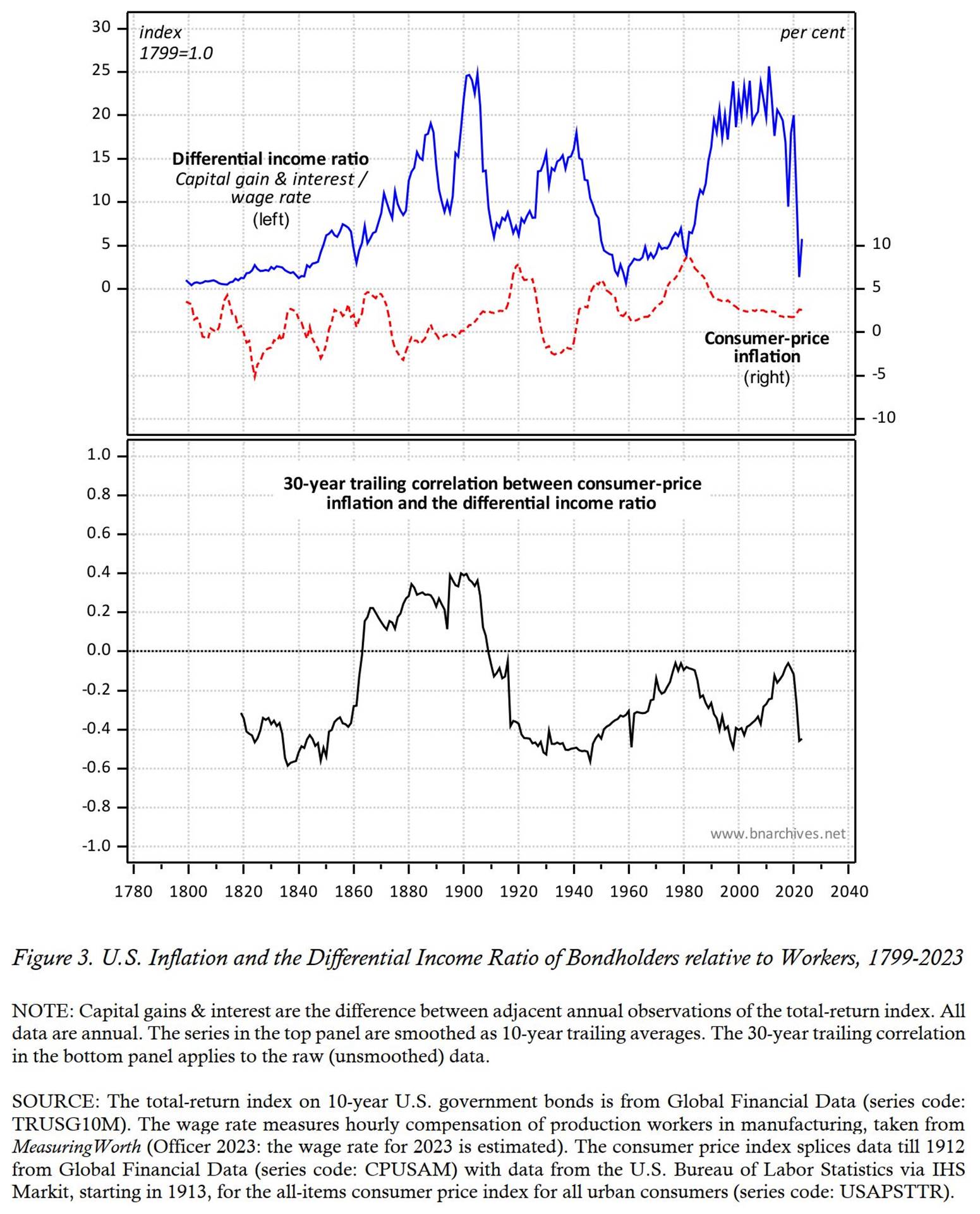
The bottom panel shows the 30-year moving correlation between the raw (i.e., un-smoothed) values of these two series. Each annual observation in this series gives the Pearson correlation coefficient in the previous 30 years. Thus, the value for 1920 expresses the correlation over the 1891-1920 period, the value for 1921 shows the correlation over the 1892-2021 period, and so on.
The chart shows that, except for the half-century between the early 1860s and 1910, the redistribution-inflation correlation has been decidedly negative. In other words, for much of its history, the U.S. saw inflation redistributing income from bondholders to workers – or more accurately, it saw inflation going together with wages rising faster (or falling more slowly) than the capital gains and interest payments received by bondholders.
Note that this picture is rather different from the one presented in Figure 5 of Fix’s article that we reproduced above. We now turn to examine this difference more closely and contemplate its reasons and implications.
7. Comparing Fix’s Results to Ours
To this point, we have presented our own view on the income distribution between bondholders and wage earners, examined how this distribution related to inflation, and considered how our findings might differ from Fix’s. However, because we use different datasets, this latter consideration was only tentative. To make it systematic, we need to disentangle the data differences from the conceptual ones, so we can concentrate on the latter only.
Start with the concepts. Fix focuses on creditors in general, whereas we examine holders of non-bearer bonds only. Next, Fix quantifies the process of creditor-worker redistribution by calculating the bond-wage growth gap – namely, the difference between the rate of growth of the bond yield and the rate of growth of wages. By contrast, we quantify this process by looking at the differential income ratio – i.e., the ratio between the total return to bondholders’ (capital gains and interest payments) and the wage rate.
Then, there are differences in the data we use. For labour income, Fix uses the wage rate earned by unskilled workers, whereas we look at the hourly compensation of manufacturing workers. And for creditors, he measures the interest yield on a basket of different 10-year fixed-income instruments spliced with 10-year government bonds, whereas we calculate the capital gains and interest earned from holding 10-year government bonds only.
Since the bone of contention is not the data but the conceptual setup, it is useful to standardize the analysis by examining both approaches with the same dataset (in this case, our own). Doing so ascertains that the differences, whatever they are, emerge from the concepts rather than the facts.
Figure 4 compares Fix’s approach to ours. The top panel shows our respective measures of creditor-worker distribution (smoothed as 30-year trailing averages, to conform with Fix’s original presentation). To reiterate, Fix measures the difference between rates of change whereas we compute the ratio of levels. In addition, Fix looks only at the bond yield, whereas we consider both capital gains and interest payments.
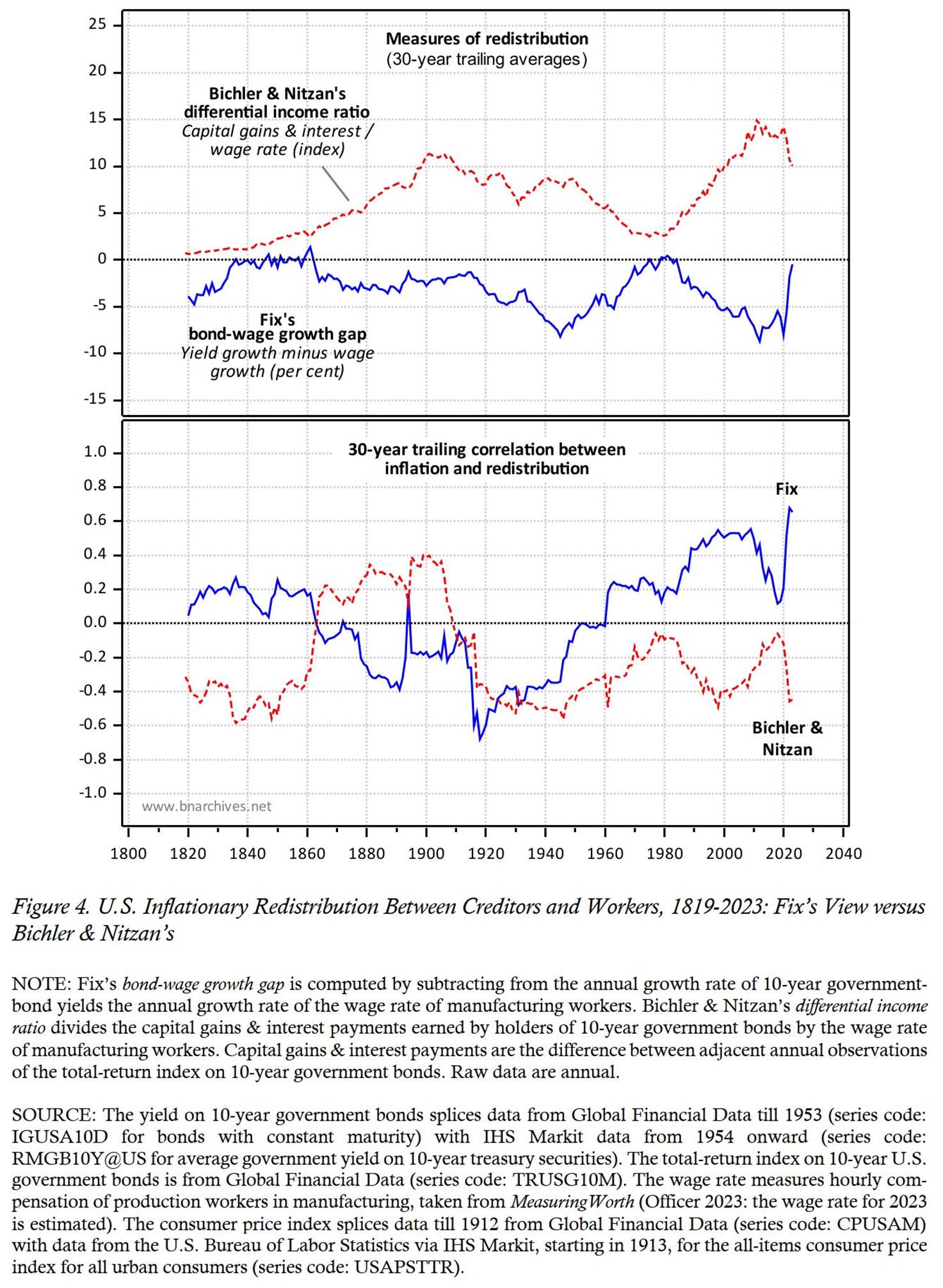
As the panel shows, the two measures tend to move inversely (their full-period correlation is -0.65). The reason lies in the mathematical relation between bond yields and bond prices. To simplify, consider a perpetual fixed-coupon bond (i.e., a bond that has no maturity date and whose interest payments do not vary). The yield on the bond is given by:
1. ![]()
And the (instantaneous) rate of change of the bond yield is determined entirely by the rate of change of its price:
2. ![]()
When the bond price increases (decreases), the yield drops (rises), and the rate of change of the latter is the exact additive inverse of the former.
This is why holders of fixed-coupon, non-bearer bonds dislike increases in the rate of interest. Note that, for existing bondholders, changes in yield have no bearing on the coupon payments they receive. These payments are fixed. Higher yields simply mean that bond prices have fallen, and lower bond prices spell capital losses.
Now, total-return indices are a bit more messy than pure bond prices primarily because they incorporate the notional ‘reinvestment’ of interest. That is why the yield’s correlation with the total return index – and by extension, its correlation with our measure of the capital gains and interest payments of bondholders – is greater than -1. But it tends to be negative, and that is why Fix’s bond-wage growth gap moves inversely with our differential income ratio.
The bottom panel of Figure 4 shows the 30-year trailing correlations between the rate of consumer price inflation on the one hand, and Fix’s and our respective distributional measures on the other. And given that Fix’s and our distributional measures move inversely, it is little surprise that their correlations with inflation move in opposite directions as well (the full-period correlation between the two 30-year correlation series is -0.25).
8. Who Sets the Rate of Interest?
The punch line in Fix’s article is monetary policymaking and its impact on the redistribution of income. Fix points out that, since the 1970s, the U.S. Fed has been fighting inflation with higher interest rates, and this policy, he argues, helped redistribute income from workers to creditors.
However, before deciding who wins and who loses from the Fed’s interest-rate policy, it is perhaps worth pondering whether we should call it a ‘policy’ in the first place.
Formally, the Fed’s interest-rate policy tool is the Federal Funds Rate, or FFR. The FFR is the overnight rate at which financial institutions lend each other, and by periodically setting its target for the FFR, the Fed is said to signal its intention to the financial market and the rest of the economy. In addition, the Fed finetunes the FFR via open market operations – either by selling bonds to drain liquidity from the market and make funds more expensive, or by buying bonds to increase liquidity and make them cheaper.
The ups and downs of the FFR, goes the argument, guide all other interest rates, from the shortest to the longest. Here is how Forbes magazine describes this process to the laity:
The federal funds rate is one of the Federal Reserve’s key tools for guiding U.S. monetary policy. It impacts everything from the annual percentage yields you earn on savings accounts to the rate you pay on credit card balances, which means the fed funds rate effectively dictates the cost of money in the U.S. economy […] The federal funds rate provides a reference for institutions as they are borrowing or lending reserves […] Fed funds is a key tool that lets the central bank manage the supply of money in the economy. That’s because it influences what banks charge each other, which informs the rates they charge you and their other customers. (Curry 2023, emphases added)
In short, the Fed is God, and its Chair and officials are Moses and the prophets.
But is this common-sense narrative valid? Does the FFR really guide the direction of market yields – or is it the other way around? In other words, could it not be that yields are determined by capitalists in the bond market and that the FFR simply echoes them?
Mind you, this is not a farfetched scenario. Many insist that Fed decisions are made independently of government intervention, but few would argue they are independent of the capitalist mode of power that the Fed is embedded in and serves. Most Fed directors represent the private member banks they come from, and its economists are selected for their impeccable neoclassical credentials. If there is anything all of them believe in, it is that the ‘market knows best’, and this common belief has consequences. If the market indeed knows best, it makes sense for monetary policy to simply parrot what has already been determined by capitalists in the prescient bond market. But then, if the Fed simply follows the market, in what sense do its actions qualify as ‘policy’, let alone as policy that determines the market rate of interest?
So how do we to discern cause from effect here? How do we know if it is the Fed that governs the market, or the market that wags the Fed? The short answer is that we do not and cannot know – at least not with any certainty. Causality is a deeply speculative ‘black box’ concept that no one can simply observe. [9] But we can proceed indirectly, by ways of tentative elimination and ranking.
One thing most would agree on is that a cause precedes its effect. If changes in the FFR cause changes in market yields, the former should come before the latter. And conversely, if changes in market yields determine changes in the FFR, variations in the former should precede those of the latter. (To avoid ambiguity, we should note that temporal precedence is a necessary but not a sufficient condition for causality: a cause X must precede its effect Y, but the fact that X precedes Y does not mean X causes Y.)
The top panel of Figure 5 begins to sort out the question by looking at the monthly history of the two processes. Specifically, we compare the FFR with the yield on 10-year government bonds (or GBY for short) – but we do so with a twist. To make the relation more apparent, we show not the actual rates, but their respective 12-month absolute per cent difference. This difference is easy to calculate: we simply subtract from the interest rate in any given month the corresponding rate a year earlier. For example, in December 2000, the FFR was 6.4 per cent, while in December 1999 it was 5.3 per cent, so the 12-month absolute per cent difference for December 2000 was 1.1 per cent (= 6.4 – 5.3). Similarly, the December 2000 value for the 10-year government-bond yield was 5.1 per cent while in December 1999 it was 6.5, which means that the 12-month absolute difference for December 2000 was -1.3 per cent (= 5.1 – 6.4).
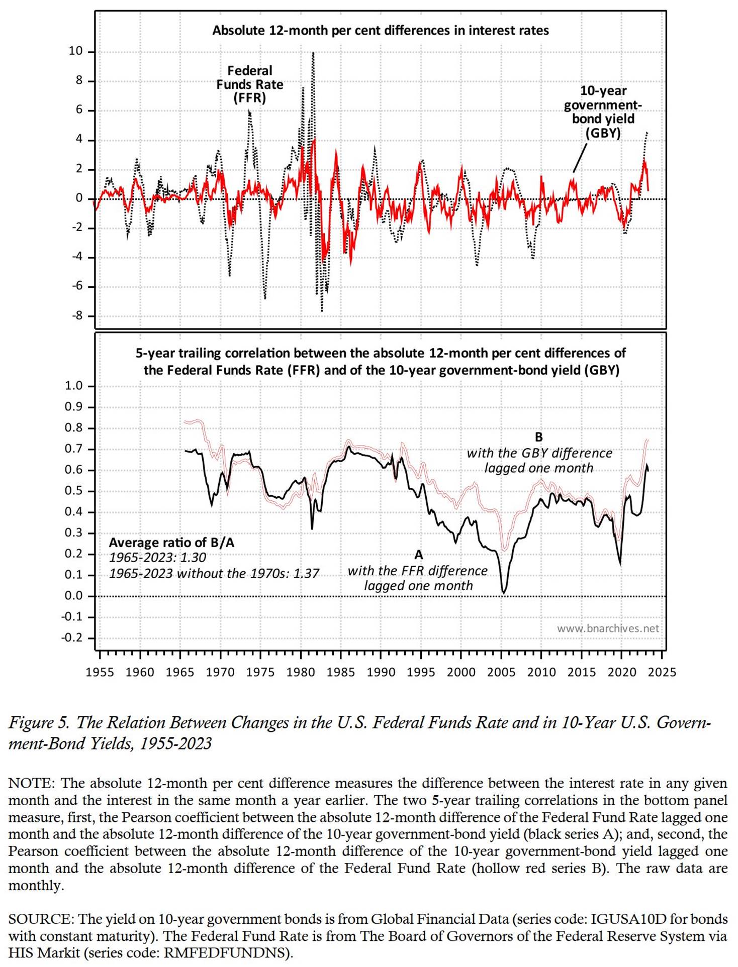
The data show that the two 12-month absolute per cent difference series share the same order of magnitude and show a similar cyclicality. But it is also evident that the relation between them tends to change over time, making it difficult to decide, at least visually, which one leads and which lags. And this is where the bottom panel becomes useful.
The bottom panel shows two 5-year trailing correlations between the two 12-month absolute per cent difference series in the top panel – with one important modification. In each case, we lag one of the series by one month. Series A (solid black) shows the correlation between the GBY and FFR differences series, with the latter series lagged by one month. [10] If changes in the FFR are the cause, they must happen before changes in the GBY; and if that is indeed the case, the correlation between them, when the FFR difference is lagged by one month, should be mostly positive. And it is. The correlation values shown by series A range between a maximum of +0.71 in 1985 and a notch over zero in 2005. And since differences in FFR lead differences GBY, it is possible that Fed policy causes the GBY to move in the same direction (we say ‘possible’, since, as noted, a statistical lead is only a necessary but not a sufficient condition for causality).
The thing is that the values of series B (hollow red), which shows the correlation with the opposite lag – i.e., between the FFR difference and the GBY difference lagged by one month – tends to be higher. Except for the 1970s, the lagged GPY difference explains the FFR difference better – and systematically so – than the lagged FFR difference explains the GPY difference! Averaged over the entire period, the correlation with GPY lagged by one month (series B) is 30 per cent higher than the correlation with the FFR lagged by one month (series A); averaged without the 1970s, it is 37 per cent higher.
Again, statistical relations, no matter how systematic, do not prove causality. But as they stand here, they put a very big dent in the seemingly impregnable belief that the Fed sets the rate of interest.
Based on our results, it appears more plausible that changes in market yields (proxied here by the GBY) are determined first and foremost by the actions of private investors and capitalist organizations that buy and sell those bonds in the market; and that, for the most part, ‘Fed policy’ simply emulates these rates by setting the FFR accordingly. [11]
From this viewpoint, it appears that, at least in the United States, the impact of interest rates on the redistribution of income and assets – whatever it may be – originates not from an independent monetary policy but from the capitalists themselves. Of course, the monetary authorities could alter the rate of interest if they so wish – according to Figure 5, they seem to have done so in the 1970s. But most of the time their ‘policy rate’ seems not to determine but to validate what capitalists have already agreed on collectively.
9. Conclusion
Let us now sum up our findings and inferences. The differences between our own results and those of Fix do not mean that our differential income ratio is correct and his bond-wage growth gap isn’t – or vice versa. The two measures quantify two different things in two different ways, and the question to consider is whether they are adequate for their stated purpose.
In his paper, Fix suggests that the goal of creditors can be represented by the bond yield, and in our view, this suggestion is too broad to be correct.
Judged by their income, creditors are not a uniform bunch. Some creditors – for example, owners of bearer bonds and bank depositors – indeed aim at the yield. But other creditors, such as financial intermediaries, are interested in the net margin between lending and borrowing rates, and still others, like holders of non-bearer bonds, are interested in the sum of capital gains and interest payments. And because their goals can differ greatly and often are opposite to one another, it is hard to speak of creditors as one social ‘class’.
According to our differential income ratio, bondholders have good reason to dislike inflation. For more than a century, they have lost from it absolutely, as well as relative to workers. And that systematic loss makes it unlikely that they will demand that governments ‘tighten’ their policy with higher interest rates – and that governments will cater to their interest by applying such policies. Other creditors with opposite interests might make such demands and even succeed in achieving them – but then, their class struggle would be with their fellow creditors as much as it would be with workers.
Moreover, claims about government monetary ‘policy’ should be made with caution. In the United States, the evidence, however tentative, suggests that the Fed does not set an independent rate of interest that lenders and borrowers then follow, but rather the opposite – namely, that the Fed follows the yield emerging from capitalist actions in the bond market.
Finally, it seems to us that the very category of ‘creditors’ has become far less useful than it once was. In the nineteenth century, classical political economists spoke about the ‘bourgeoisie’ and distinguished ‘industrial capitalists’ from ‘commercial capitalists’, ‘rentiers’ and ‘financiers’, while in the early twentieth century Keynes still separated ‘savers’ from ‘investors’. But in contemporary capitalism, these categories and divisions have become anachronistic and often impossible to concretize. Leading investors and capitalist organizations – or what we call ‘dominant capital’ – are not only grouped in hierarchical alliances and interlocked with government organs, but their incomes derive from the full spectrum of investment instruments. They are almost always both creditors and debtors, as well as owners of equities, currencies, commodities and whatnot. Ultimately, it is this intertwined hierarchy of power that must be examined if we are to decipher redistribution in general and inflationary redistribution in particular.
Endnotes
[1] Shimshon Bichler and Jonathan Nitzan teach political economy at colleges and universities in Israel and Canada, respectively. All their publications are available for free on The Bichler & Nitzan Archives (https://bnarchives.net).
[2] For selected CasP works on inflationary redistribution, see Ali (2011), Baines (2014a, 2014b), Bichler and Nizan (2004, 2015, 2021), Fix (2022), Mouré (2023), Nitzan (1992) and Nitzan and Bichler (1995, 2001; 2002: Ch. 4; 2009: Ch. 16).
[3] For in-depth discussions of these issues, see Nitzan (1992: Ch. 5), Nitzan and Bichler (2009: Ch. 8), Fix (2019) and Fix, Bichler and Nitzan (2019).
[4] Fix (2021, 2022, 2023a, 2023b, 2023c, 2023d, 2023e, 2023f, 2023g). Fix’s research is available from his Creative Commons website, Economics from the Top Down https://economicsfromthetopdown.com.
[5] A bond is typically issued with a ‘par value’, which is the money the bondholder will receive when the bond matures, and a ‘coupon rate’, which is the bondholder’s periodic interest payment, expressed as a per cent of the bond’s par value. For example, if the par value is $1,000 and the annual coupon rate is 3 per cent, the bondholder will receive $30 a year in interest till the bond matures. Normally, the par value and coupon rate – and therefore the coupon dollar payment – do not change for the duration of the bond. By contrast, the market price of a (non-bearer, traded) bond fluctuates and usually differs from its par value.
[6]
To illustrate, suppose that, in period 1, the price of
the bond is $100; that in period 2 the price is still $100 but the bondholder
receives a coupon payment of $10; and that in period 3 the bond price rises by
10 per cent to $110. In the agency’s calculation,
the bond’s total-return index will be 100 in period 1, 110 in period 2 (= 100 +
10) and 121 in period 3 ![]() .
.
[7] Bond indices are designed to reflect the price and yield corresponding to their stated maturity. Thus, a 10-year government bond index should reflect the price and yield of government bonds maturing in ten years, while a 5-year corporate bond index should reflect those of corporate bonds maturing in five years. To do so, the data agency constantly replaces the bonds it tracks to keep the effective maturity of the index as close as possible to its stated one. The different bonds in the index are commonly weighed by their market value, though other weights can be used too.
[8] Recall that Fix uses the wage rate of unskilled workers. We prefer the broader and perhaps more representative compensation of workers in manufacturing. Over the period in question, the manufacturing wage rate rose 2.5 times faster than that of unskilled workers.
[9] For a glimpse of the complexities and circularities invoked by causality, see Bunge (1961, 1979).
[10] To illustrate, the observation for December 2000 is the correlation between the 60 observations of the GBY difference ranging from January 1996 to December 2000 and the 60 observations of the FFR difference ranging from December 1995 to November 2000 (i.e., the FFR difference series lagged by one month). Similarly, the observation for January 2001 correlates the February 1996-January 2001 window for the GBY difference with the January 1996-December 2000 for the FFR difference, and so on.
[11] Safeguarding the Fed’s honour, mainstream economists might dismiss our presentation as naïve misunderstanding. The rate of interest, they would argue, is set by the Fed’s FFR. That’s the undisputed truth. And while the GBY difference indeed precedes the FFR one, that is because the market correctly anticipates the Fed’s policy! The problem is that making such argument would validate its very opposite – namely, that changes in the rate of interest are determined by capitalists in the market, and that the Fed simply anticipates the market correctly. . . .
References
Adams, Robert, Vitaly M. Bord, and Bradley Katcher. 2022. Credit Card Profitability. Washington: Board of Governors of the Federal Reserve System. FEDS Notes (September 9).
Ali, Syed Ozair. 2011. Power, Profits and Inflation: A Study of Inflation and Influence in Pakistan. State Bank of Pakistan. SBP Working Paper Series (43, December): 1-23.
Baines, Joseph. 2014a. Food Price Inflation as Redistribution: Towards a New Analysis of Corporate Power in the World Food System. New Political Economy 19 (1, January): 79-112.
Baines, Joseph. 2014b. Wal-Mart's Power Trajectory: A Contribution to the Political Economy of the Firm. Review of Capital as Power 1 (1): 79-109.
Bichler, Shimshon, and Jonathan Nitzan. 2004. Dominant Capital and the New Wars. Journal of World-Systems Research 10 (2, August): 255-327.
Bichler, Shimshon, and Jonathan Nitzan. 2015. Still About Oil? Real-World Economics Review (70, February): 49-79.
Bichler, Shimshon, and Jonathan Nitzan. 2021. Relative Oil Prices and Differential Oil Profits. Real-World Economics Review Blog, December 30.
Curry, Benjamin. 2023. Understanding the Federal Funds Rate. Forbes Advisor, April 12.
Ennis, Huberto M., Helen Fessenden, and John R. Walter. 2016. Do Net Interest Margins and Interest Rates Move Together? Federal Reserve Bank of Richmond Economic Brief (May): 1-6.
Fix, Blair. 2019. The Aggregation Problem: Implications for Ecological and Biophysical Economics. BioPhysical Economics and Resource Quality 4 (1): 1-15.
Fix, Blair. 2021. The Truth About Inflation. Economics from the Top Down, November 24.
Fix, Blair. 2022. Inflation: Everywhere and Always Differential. Economics from the Top Down, pp. 1-17.
Fix, Blair. 2023a. The Cause of Stagflation. Economics from the Top Down, January 26, pp. 1-15.
Fix, Blair. 2023b. Do High Interest Rates Reduce Inflation? A Test of Monetary Faith. Economics from the Top Down, February 4, pp. 1-18.
Fix, Blair. 2023c. How Interest Rates Redistribute Income. Economics from the Top Down, April 16, pp. 1-31.
Fix, Blair. 2023d. Inflation! The Battle Between Creditors and Workers. Economics from the Top Down, March 23, pp. 1-20.
Fix, Blair. 2023e. Interest Rates and Inflation: Knives Out. Economics from the Top Down, February 19, pp. 1-29.
Fix, Blair. 2023f. Is Stagflation the Norm? Economics from the Top Down, January 17, pp. 1-19.
Fix, Blair. 2023g. The Key to Managing Inflation: Higher Wages. Economics from the Top Down, March 2, pp. 1-15.
Fix, Blair, Shimshon Bichler, and Jonathan Nitzan. 2019. Real GDP: The Flawed Metric at the Heart of Macroeconomics. Real-World Economics Review (88, July): 51-59.
Mouré, Christopher. 2023. Technological Change and Strategic Sabotage: A Capital as Power Analysis of the US Semiconductor Business Real-World Economics Review (103, March): 26-55.
Nitzan, Jonathan. 1992. Inflation as Restructuring. A Theoretical and Empirical Account of the U.S. Experience. Unpublished PhD Dissertation, Department of Economics, McGill University.
Nitzan, Jonathan, and Shimshon Bichler. 1995. Bringing Capital Accumulation Back In: The Weapondollar-Petrodollar Coalition -- Military Contractors, Oil Companies and Middle-East "Energy Conflicts". Review of International Political Economy 2 (3): 446-515.
Nitzan, Jonathan, and Shimshon Bichler. 2001. Going Global: Differential Accumulation and the Great U-turn in South Africa and Israel. Review of Radical Political Economics 33 (1): 21-55.
Nitzan, Jonathan, and Shimshon Bichler. 2002. The Global Political Economy of Israel. London: Pluto Press.
Nitzan, Jonathan, and Shimshon Bichler. 2009. Capital as Power. A Study of Order and Creorder. RIPE Series in Global Political Economy. New York and London: Routledge.
Officer, Lawrence H. 2023. Characteristics of the Production-Worker Compensation Series. In MeasuringWorth.org.
Samuelson, Paul A., and William D. Nordhaus. 2010. Economics. 19th ed. Boston: McGraw-Hill Irwin.